
Background
Artificial Intelligence: Possibilities and Limitations
Since the conception of Artificial intelligence, scientists and engineers have tried to artificially replicate every human skill, and many attempts to achieve them have been successful to some extent. We now have robots capable of running, jumping and doing specific manual labor; autonomous vehicles able to navigate and avoid obstacles with near-human perception; algorithms and simulations that allow scientist to better understand the laws of physics that governs us, the biological processes of living organisms, and several other applications in different fields and industries like finance, commerce, healthcare, education, public policy, and more. However, all of these applications have something in common: they rely on numerical analysis, pattern recognition and other analytical processes. However, despite these limitations, the question on whether human mind will be surpassed by AI is no longer if it will happen, but when it will happen.
 Will human mind be surpassed by AI? |
The advent and development of Machine learning and Deep Neural Networks has caused many AI pioneers and authorities to debate whether machines will be capable of reaching the pinnacles of human mind: innovation, creativity, and imagination. As we just presented it, AI & ML applications have the ability to infer results mostly on pattern recognition and task replication, but little progress on cognitive process simulations has been achieved. However, this does not mean that that it won’t happen, but it is clear that there is a long way in research and innovation to go. In this project, we will explore one of the most well-known attempts to replicate human visual artistic creativity using common machine learning techniques.
Neural Networks: The 21st Century Prime Artists?
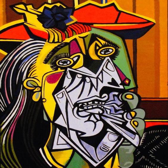
Humans, like no other species, have been gifted with outstanding creativity which has been an invaluable tool not just to solve problems but to express complex and abstract ideas. For centuries, people have relied on painting as a way to convey knowledge, events, and feelings. Over time, painting techniques have been evolving and perfecting and several and although many artists have produced meaningful masterpieces, few are considered to have reached excellence based on multiple factors: Leonardo da Vinci, Vincent van Gogh, Pablo Picasso, and Salvador Dalí, just to mention a few. Within the realm on AI there has been attempts to recreate the creative process with little success. However, the dawn of computer vision and convolutional neural networks (CNN) have allowed the creation of alternatives with pretty amazing results: Artistic Style Transfer.
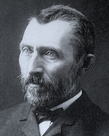 Illustrious artist. |
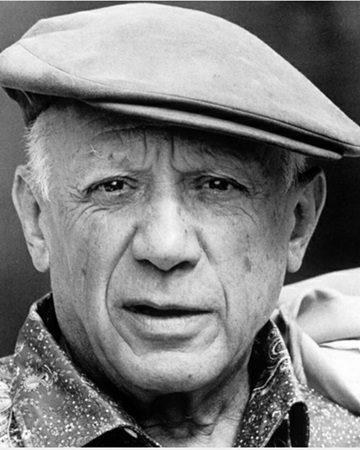 Illustrious artist. |
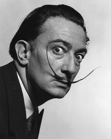 Illustrious artist. |
Although neural networks are not yet capable to produce original works of art, they are pretty good in replicating the style of current works of art. Artistic style transfer is the technique of recomposing images in the style of other images, usually paintings. This novel technique was developed and published by a team of computer scientist and neuroscientist at the Bethge Lab in the University of Tübingen, Germany. In this project, we implement the research paper: A Neural Algorithm of Artistic Style by L. A. Gatys, A. S. Ecker, M. Bethge, et al. This algorithm is based on an artificial system grounded on a Deep Neural Network, which ultimately will generate artistic images of “high perceptual quality.”
Convolutional Neural Networks & Style Transfer Overview
Convolutional Neural Networks overview
Convolutional Neural Networks (CNNs) are a category of Neural Networks that are effective to solve computer vision problems such as image classification and image recognition. The are commonly used to detect faces, moving object such as cars in highways, and other similar applications. They are made up of “neurons” that have learnable weights and biases. Usually, convolutional neural networks take an image as an input, performs some convolutions (dot products) using kernels (filters), and optionally follows it with a with a non-linearity activation function such as ReLU (rectified linear unit).
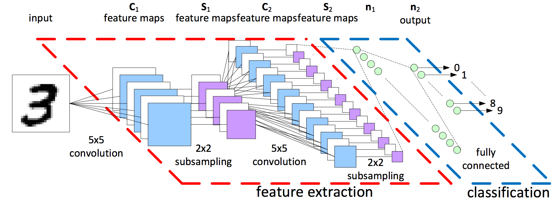 A generic CNN for numeric recognition. The model is similar for other vision recognition tasks. (PyLessons.com). |
In standard classification problems, once the image data has reached the last convolutional layer then it is converted into a suitable form (usually just flattening the date into a one-dimensional vector) for a fully connected layer, which is also known as a Multi-Level Perceptron. The flattened data is then fed to a feed-forward neural network and backpropagation applied to every iteration of training. After a series of training loops, or epochs, the model “learns” to distinguish certain features in images.
 A generic CNN for numeric classification. |
In this project, however, we won’t need the fully connected layer to generate the image. The reason is that we are not interested in classifying images, but on the convolution results of some layers from a standard (but modified) VGG network architecture. To learn more about convolution neural networks, please visit the overview section of Project 4: Facial Keypoint Detection with Neural Networks.
Neural Style Transfer Overview
Neural Style Transfer is a technique where we can stylize an input image based on the style of another image, while preserving the content of the original input image. Convolutional neural networks contain many layers, and each layer can be understood as a collection of image filters, each of which extracts a certain feature from the input image (Gatys). The output of a given layer are knows feature maps since each one contains a filtered version of the same input image. We could use these intermediate layers to extract the features or content from the first image, and the style from the second image. Then we combine these results to produce a final stylized image, thus concluding the style transfer. The problem is then is reduced to tree steps: obtaining the content and style and combining them to produce a visually appealing result.
|
Using a modified CNN to extract the content from first image to be stylized and style from the artwork to be replicated. |
Extracting the image content
In a convolutional neural network, as an image moves deeper into the network hierarchy, the features or content becomes more prominent (see diagram below). In other words, “higher layers in the network capture the high-level content in terms of objects and their arrangement in the input image but do not constrain the exact pixel values of the reconstruction” (Gatys). This information can be used to reconstruct an approximation of input image, although not necessarily to pixel-by-pixel accuracy. This will be useful when generating the final output image.
Content Reconstructions.
Gatys states that we can visualize the information at different processing stages in the Convolutional Neural Network by reconstructing the input image just by knowing the network’s responses in a particular layer. In the diagram above, we can see a sequence of different versions of the reconstructed content image (Neckarfront houses) from layers “conv1_1” (a), “conv2_1” (b), “conv3_1” (c), “conv4_1” (d) and “conv5_1” (e) of the original CNN (The author used a VGG network architecture which stands for Visual Geometry Group). Note that the reconstructions from lower layers (a), (b), and (c) of the CNN are almost perfect, while the reconstructions from higher layers (d) and (e) are able to retain the high-level content of the image, but detailed pixel-to-pixel information is lost.
Extracting the image style
This step is a bit tricker since the style cannot be inferred from the convolutional layer directly. In order to get the representations of the image style, it is necessary to compute the correlations between different types layers in the network using the Gram Matrix. The Gram-matrix is essentially just a matrix of dot-products for the vectors of the feature activations of a style-layer. By doing so, “we obtain a stationary, multi-scale representation of the input image, which captures its texture information but not the global arrangement” (Gatys). In other words, we can achieve the best style representation by combining the textures of many different layers from the convolutional neural network.
Style Reconstructions
To get an accurate style representation we need to compute the correlations between the different features in different layers of the CNN. Gatys and his team were able to reconstruct the style of the input image from style representations (correlations) built on different subsets of CNN layers:
- “conv1_1”
- “conv1_1” and “conv2_1”
- “conv1_1”, “conv2_1” and “conv3_1”
- “conv1_1”, “conv2_1”, “conv3_1” and “conv4_1”
- “conv1_1”, “conv2_1”, “conv3_1”, “conv4_1” and “conv5_1”
These combined results recreate images that match the style texture on the original style image on an increasing scale (as we can see in the diagram above), while removing information of the overall arrangement and content of the original image. In the next section we delve deeper into the mathematical basis and implementation of this net.
Network Architecture Implementation
Setting up the VGG-19 architecture
The first step is to setup the convolutional neural network. We will use the first 16 layers of the VGG-19 architecture as suggested by the authors (we don’t need to fully connected layer). VGG models are pretty sophisticated and large Neural Network models with convolutional layers whose performance in object identification is comparable to human performance. These models are trained for prolongated periods of times (days to weeks) using state-of-the-art GPUs. Fortunately, trained models are readily available in major open-source computer vision and machine learning libraries such as PyTorch.
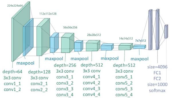 VGG-19 architecture. (Clifford K. Yang) |
The original VGG network model from PyTorch is the following:
Sequential(
  (0): Conv2d(3, 64, kernel_size=(3, 3), stride=(1, 1), padding=(1, 1))
  (1): ReLU(inplace=True)
  (2): Conv2d(64, 64, kernel_size=(3, 3), stride=(1, 1), padding=(1, 1))
  (3): ReLU(inplace=True)
  (4): MaxPool2d(kernel_size=2, stride=2, padding=0, dilation=1, ceil_mode=False)
  (5): Conv2d(64, 128, kernel_size=(3, 3), stride=(1, 1), padding=(1, 1))
  (6): ReLU(inplace=True)
  (7): Conv2d(128, 128, kernel_size=(3, 3), stride=(1, 1), padding=(1, 1))
  (8): ReLU(inplace=True)
  (9): MaxPool2d(kernel_size=2, stride=2, padding=0, dilation=1, ceil_mode=False)
  (10): Conv2d(128, 256, kernel_size=(3, 3), stride=(1, 1), padding=(1, 1))
  (11): ReLU(inplace=True)
  (12): Conv2d(256, 256, kernel_size=(3, 3), stride=(1, 1), padding=(1, 1))
  (13): ReLU(inplace=True)
  (14): Conv2d(256, 256, kernel_size=(3, 3), stride=(1, 1), padding=(1, 1))
  (15): ReLU(inplace=True)
  (16): Conv2d(256, 256, kernel_size=(3, 3), stride=(1, 1), padding=(1, 1))
  (17): ReLU(inplace=True)
  (18): MaxPool2d(kernel_size=2, stride=2, padding=0, dilation=1, ceil_mode=False)
  (19): Conv2d(256, 512, kernel_size=(3, 3), stride=(1, 1), padding=(1, 1))
  (20): ReLU(inplace=True)
  (21): Conv2d(512, 512, kernel_size=(3, 3), stride=(1, 1), padding=(1, 1))
  (22): ReLU(inplace=True)
  (23): Conv2d(512, 512, kernel_size=(3, 3), stride=(1, 1), padding=(1, 1))
  (24): ReLU(inplace=True)
  (25): Conv2d(512, 512, kernel_size=(3, 3), stride=(1, 1), padding=(1, 1))
  (26): ReLU(inplace=True)
  (27): MaxPool2d(kernel_size=2, stride=2, padding=0, dilation=1, ceil_mode=False)
  (28): Conv2d(512, 512, kernel_size=(3, 3), stride=(1, 1), padding=(1, 1))
  (29): ReLU(inplace=True)
  (30): Conv2d(512, 512, kernel_size=(3, 3), stride=(1, 1), padding=(1, 1))
  (31): ReLU(inplace=True)
  (32): Conv2d(512, 512, kernel_size=(3, 3), stride=(1, 1), padding=(1, 1))
  (33): ReLU(inplace=True)
  (34): Conv2d(512, 512, kernel_size=(3, 3), stride=(1, 1), padding=(1, 1))
  (35): ReLU(inplace=True)
  (36): MaxPool2d(kernel_size=2, stride=2, padding=0, dilation=1, ceil_mode=False)
)
The final network architecture after the modifications specified by Gatys et al. is the following:
Sequential(
  (0): Normalizer()
  (conv_1): Conv2d(3, 64, kernel_size=(3, 3), stride=(1, 1), padding=(1, 1))
  (styleL_1): styleLoss()
  (relu_1): ReLU()
  (conv_2): Conv2d(64, 64, kernel_size=(3, 3), stride=(1, 1), padding=(1, 1))
  (styleL_2): styleLoss()
  (relu_2): ReLU()
  (pool_2): MaxPool2d(kernel_size=2, stride=2, padding=0, dilation=1, ceil_mode=False)
  (conv_3): Conv2d(64, 128, kernel_size=(3, 3), stride=(1, 1), padding=(1, 1))
  (styleL_3): styleLoss()
  (relu_3): ReLU()
  (conv_4): Conv2d(128, 128, kernel_size=(3, 3), stride=(1, 1), padding=(1, 1))
  (contentL_4): contentLoss()
  (styleL_4): styleLoss()
  (relu_4): ReLU()
  (pool_4): MaxPool2d(kernel_size=2, stride=2, padding=0, dilation=1, ceil_mode=False)
  (conv_5): Conv2d(128, 256, kernel_size=(3, 3), stride=(1, 1), padding=(1, 1))
  (styleL_5): styleLoss()
)
And the hyperparameters that we found to produce good results are shown below. Note that for every image and style the parameters were adjusted to produce the most appealing results.
- Output size: (256 x 256) and (512 x 525) pixels
- Ratio α/β: 1x10⁻⁴ to 1x10⁻⁶
- Number of steps: 300 to 1000
Content Loss
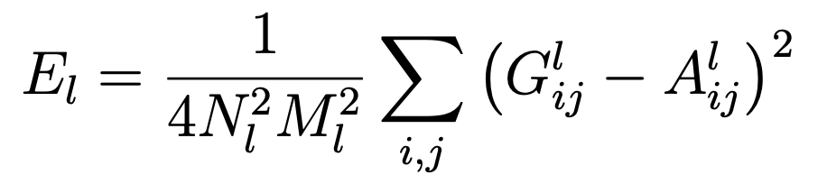
Once we have downloaded the pre-trained model we proceed to modify as suggested by the author. For the VGG content layer “conv_4” we define a special loss function defined as follows: given an input image x, the CNN will encode it into its layers by using the filter responses from that image. A layer with Nl distinct filters has Nl feature maps each of size Ml, where Ml is the number of “neurons” contained in that layer grid. The responses in a layer l can be stored in a matrix Fl ∈ RNl×Ml where Flij is the activation of the ith filter at position j in layer l. In other words, Fl denotes the representation of the optimization image at layer l of the CNN. Then, we can define the content loss function as follows:
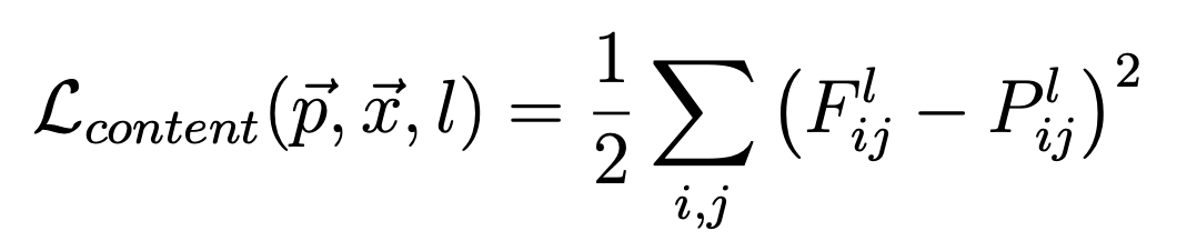 Content loss. |
- p represents the original content image
- x represents the synthetized image
- l represents the current layer
- Flij represents the activation of the ith filter at position j in the feature representation of x in l
- Plij represents the activation of the ith filter at position j in the feature representation of p in l
The equation above states that the content loss generated at layer l of our CNN with regards to a content image p and an optimization image x, is the average square difference between each content representation, or activation, of p and x at layer l.
Style Loss
Additionally, we need to modify the layers “conv_1”, “conv_2”, “conv_3”, “conv_4”, and “conv_5” to “built a style representation that computes the correlations between the different filter responses, where the expectation is taken over the spatial extend of the input image” (Gatys). For it we will need to use a Gram matrix and since it is a bit tricky to understand what it does, we present a brief explanation and one example before moving on.
The Gram Matrix
As we previously mentioned, the Gram matrix manages to capture the general style of an image while reducing the overall features from the image. In order to learn the style of the given art picture, we need to measure which features in the style-layers activate simultaneously for the style-image, so we can use this activation-pattern on the final synthetized image. To do this, we calculate the Gram matrix, which is basically a matrix of inner products between the vectorized feature maps. To better understand how it works we present a toy example. Let x be a flattened feature map (for simplicity, we use 1 x 3 map containing M=3 pixels). Note that at the beginning, x is the original image.
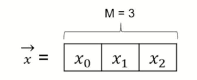 A flattened feature map example. |
Then, we apply a sequence of filters Zi to x, and the result will be a C x H x W tensor of features (H x W grid of C dimensional vectors). In this example, C = 2 filters, and H x W = 1 x 3. The resulting matrix (or tensor) after applying the filters Z0 and Z1 are the following:
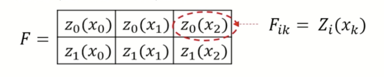 Filtered featured map. |
As we can see, the more filters we apply will increase the “volume” of the tensor. The next step is selecting two of these different feature vectors (see pink and blue dimensional vectors below), and we compute the outer product between them (thus each entry is an inner product of the elements of the pink and blue dimensional vectors).
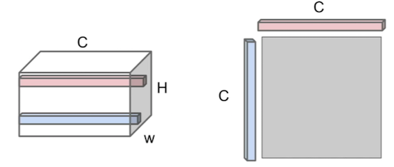 Outer product between feature vectors. |
The resulting C x C = 2 x 2 matrix contains information about which features in that feature map tend to activate together at those two specific spatial positions.
 Gram Matrix. |
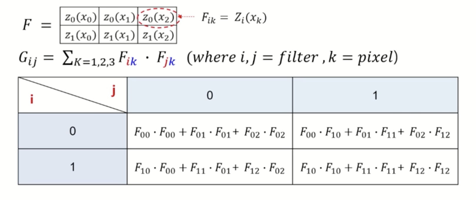
A generalization of this example for our CNN can be expressed as follows:
 Gram Matrix equation for style transfer. |
- Gij represents the inner product between the vectorized featured map i and j in layer l
- Fik represents the activation of the ith filter at pixel position k in the flat feature representation in layer l
- Fjk represents the activation of the jth filter at pixel position k in the flat feature representation in layer l
Note that If an entry in the Gram matrix has a value close to zero then it means the two features in the given layer do not activate simultaneously for the given style-image. Conversely, if an entry in the Gram matrix has a large value, then it means the two features do activate simultaneously for the given style-image.
Style Loss (continued)
Now that we know how the Gram matrix work, we can move forward with the implementation of the style loss. According to the authors, in order to produce a texture that matches the style of a given image, we need to use gradient descent from a white noise image, or alternatively, the original content image, to generate an image that matches the style representation of the original style image. We can accomplish this by minimizing the mean-squared distance between the entries of the Gram matrix from the original style image (the artwork picture) and the Gram matrix of the image being generated (the stylized image). Consider a be the original artwork image and x be the image being generated by our CNN, and Al and Gl be their respective style representations in layer l. Then, the contribution of that layer to the total loss is represented as:
 Loss contribution for layer l. |
- Nl represents the number of feature maps
- Ml represents the flattened dimension of the feature map grid (Height x Width)
- Glij represents the pairwise feature maps i and j in the style representation of original image x in layer l
- Alij represents the pairwise feature maps i and j in the style representation of generated image a in layer l
Then we apply the style loss function on the different layers to get the total style loss:
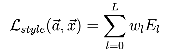 Style Loss. |
- a represents the original artwork image
- x represents the image being generated
- L represents the number of activation layers
- wl represents the weighting factors of the contribution of each layer to the total loss
- El represents the loss in current layer l
The gradients of El with respect to the activations in lower layers of the network can be readily computed using standard error back-propagation. We conveniently use the backward() function from PyTorch’s nn.module to achieve this.
Total Loss
Finally, in order to generate the final stylized image, we minimize the distance error from it to both the content representation of the original image and the style in the artwork style. Therefore, the total loss can then be written as a weighted sum of the both the style and content losses as shown below.
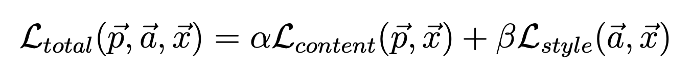 Total Loss. |
The hyperparameters α and β are used to adjust the balance between content and style for the output. Although the author suggests that good results can be achieved when the ratio α/β is between either 1×10⁻³ or 1x10⁻⁴, we found that best result in our implementations can be achieved when using a ratio 1x10⁻⁶. With this we completed the implementation and now we are ready to show off some results!
Results and Analysis
Neckarfront: Expected vs actual results
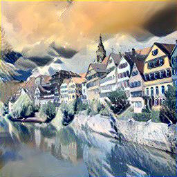
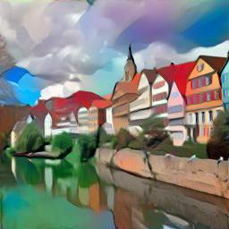
Now that we have our Neural Style Transfer Network implemented, we can try it to generate images that combine the content representation of an image. In order to compare our results with the ones provided in the paper, we will transfer different well-known paintings styles into a photo of the “Neckarfront” a location in Tubingen, Germany.
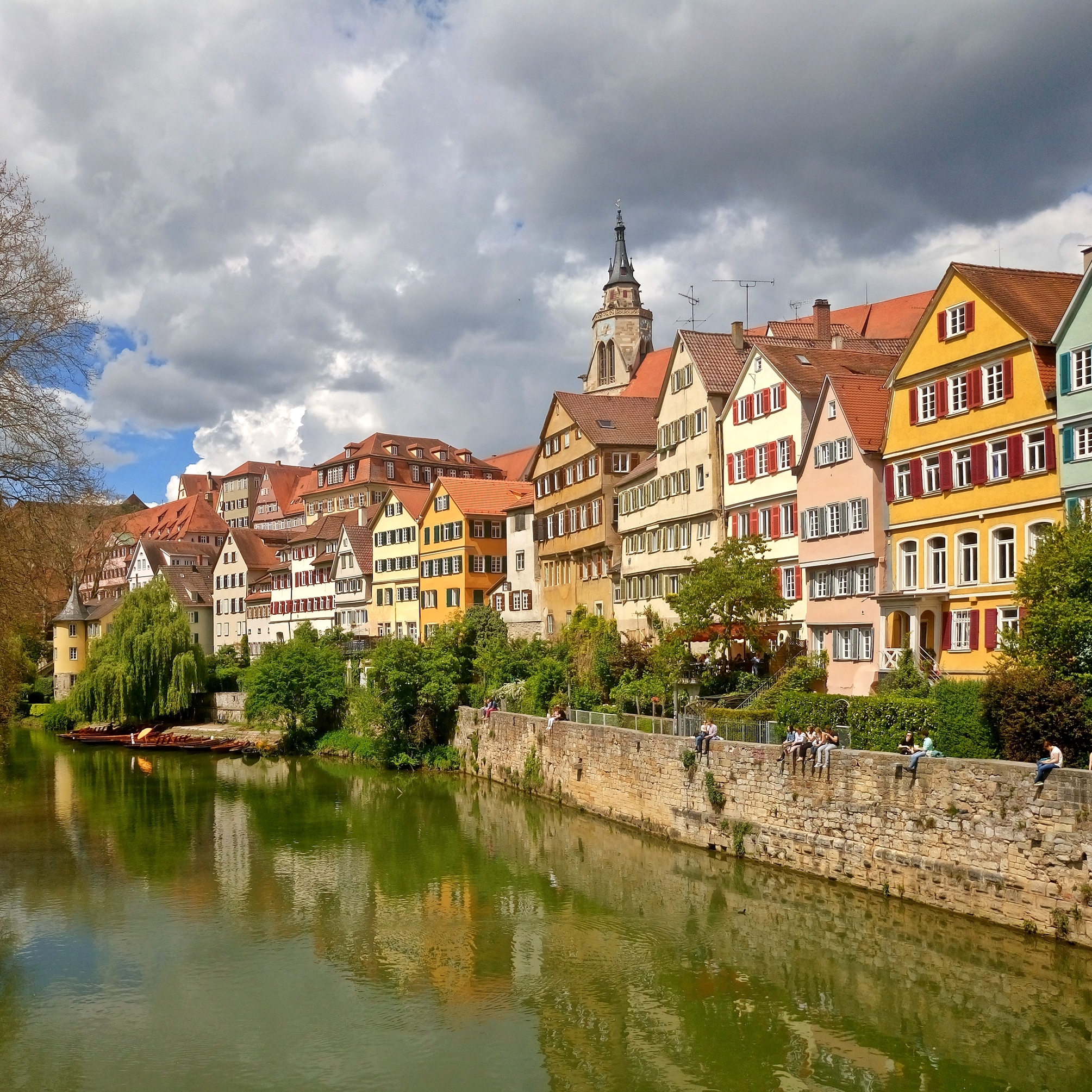 “Neckarfront” a location in Tubingen, Germany. |
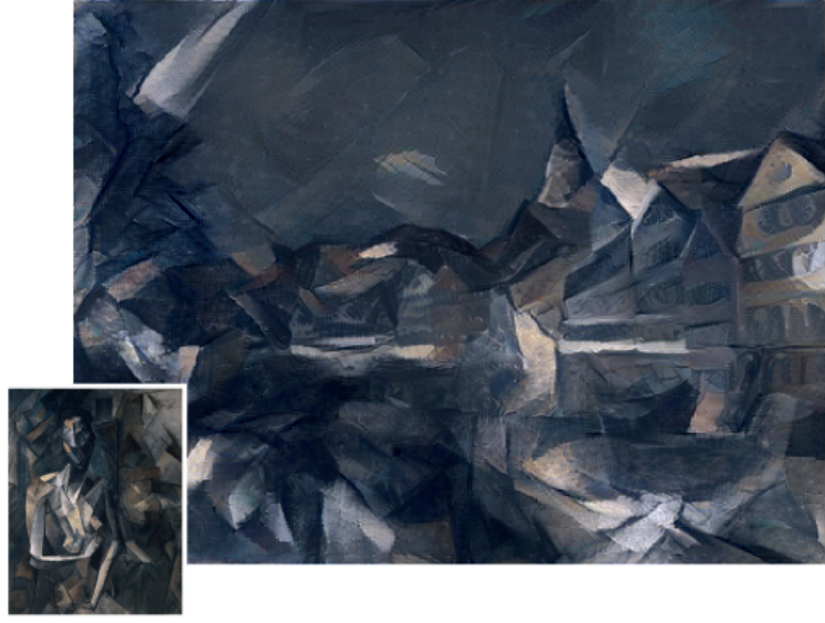
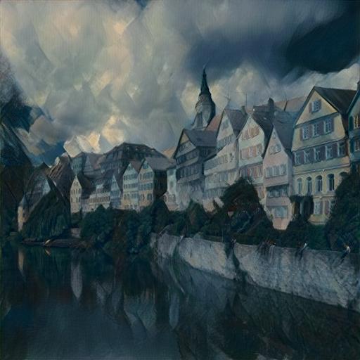
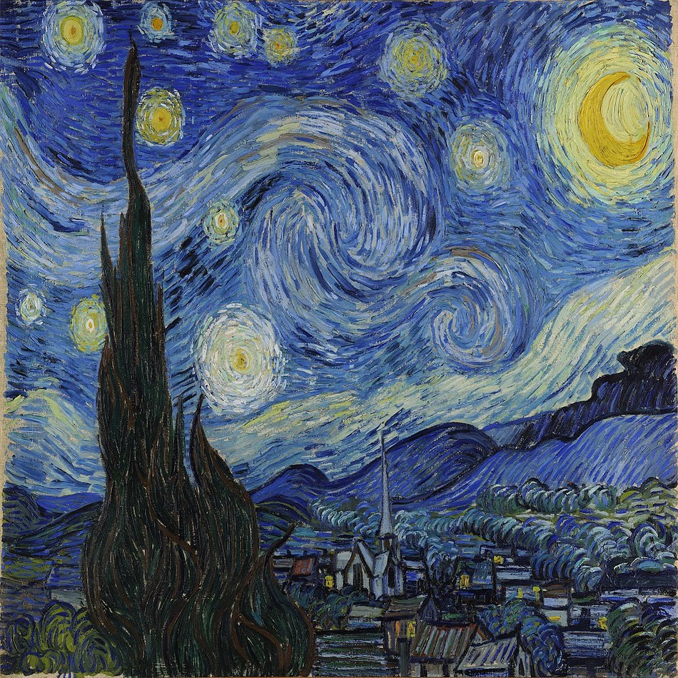
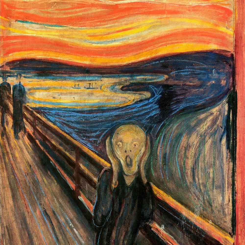
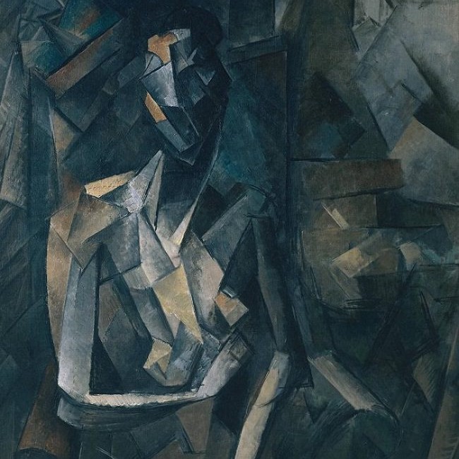
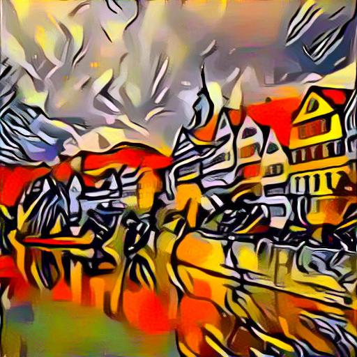
It is worth mentioning that depending on the complexity and level of abstraction of the selected artwork, the amount of detail on the synthetized image can vary significantly. For example, the stylized image based on “The Starry Night” by Vincent van Gogh has more fine details than the stylized image based on “The Scream” by Edvard Munch. However, the loss function we use for the style transfer contains two terms representing the content and style. We can therefore control the emphasis on content or the style when synthesizing the image. We present these results below and we include some additional artwork styles: “The shipwreck of the Minotaur” by Mallord William Turner and "Seated Nude" (Femme Nue Assise) by Pablo Picasso.
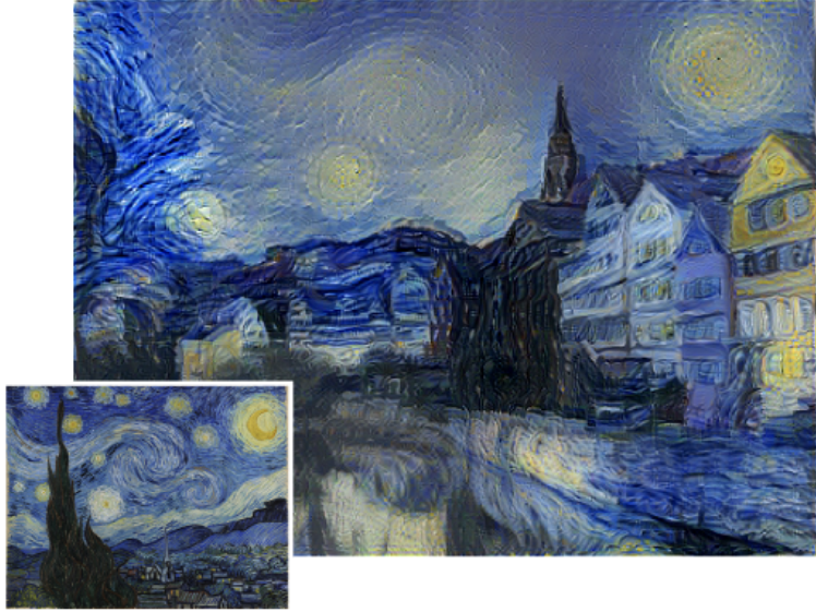 Generated version from Gatys et al. paper. |
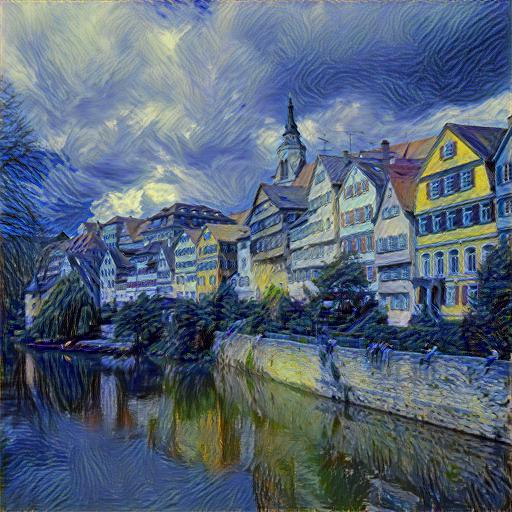 Our generated version. |
|
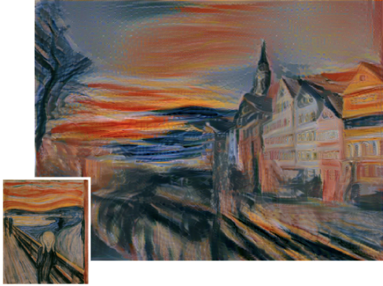 Generated version from Gatys et al. paper. |
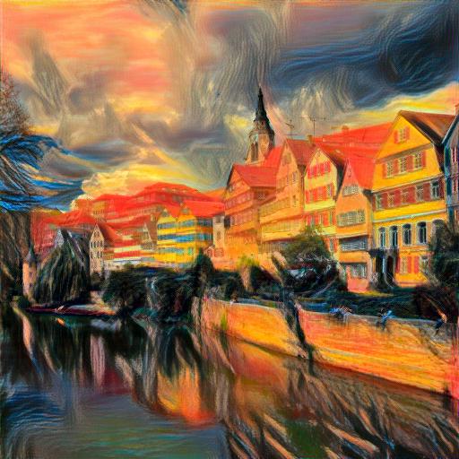 Our generated version. |
|
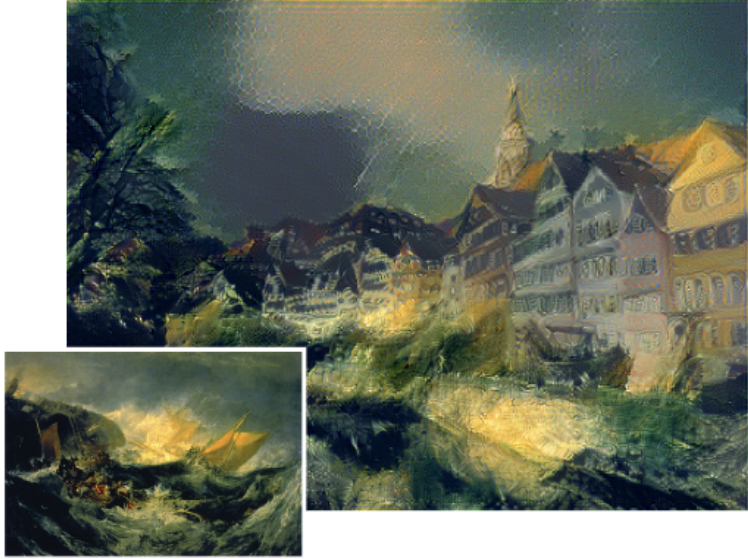 Generated version from Gatys et al. paper. |
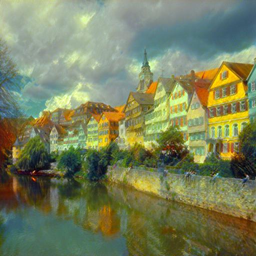 Our generated version. |
|
 Generated version from Gatys et al. paper. |
 Our generated version. |
|
As we can see, the original content of the photograph is preserved while the colors, mood, and the texture is provided by the artwork. Our results, however, retain more information about the content of the Neckarfront photo. This is probably because our α/β (content/style) ratio was a bit different to the exact ratio that the authors decided on the final results. This transfer technique is so effective that it really seems as if the original artist painted them. However, these outstanding results just show the remarkable flexibility and power of convolutional neural networks. If we go back to our early discussion on AI and creativity, we could be tempted to claim that CNNs have actually achieved creative abilities based on above results, but they have not. In reality, this CNN specifically designed to extract features from provided images by us. A truly creative artificial entity would generate similar results based on its knowledge about the world (scenery, objects, people, etc.) and a hit of imagination for the style (maybe inspired by looking at other artworks). There have been some examples of so-called “real” art generated by AI. The most famous piece of art (as of Dec 2020) was “Edmond de Belamy”, an abstract portrait generated a GAN (Generative Adversarial Network) which was designed by Paris-based arts-collective Obvious in 2018 and sold for nearly half million dollars! Click here see more AI artworks from the original researchers.
Art Gallery
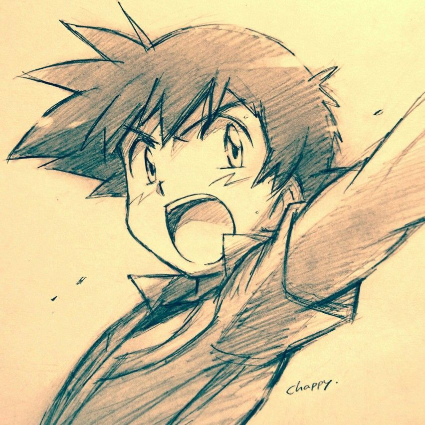
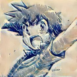
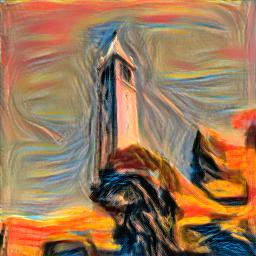
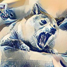
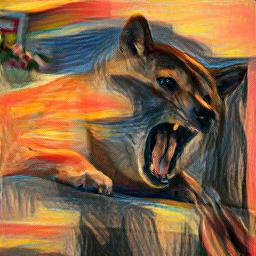
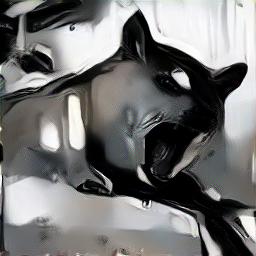
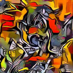
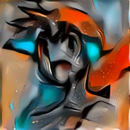
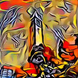
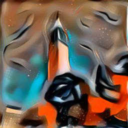
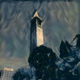
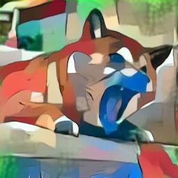
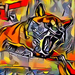
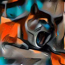
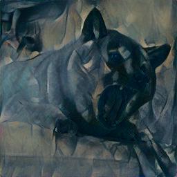
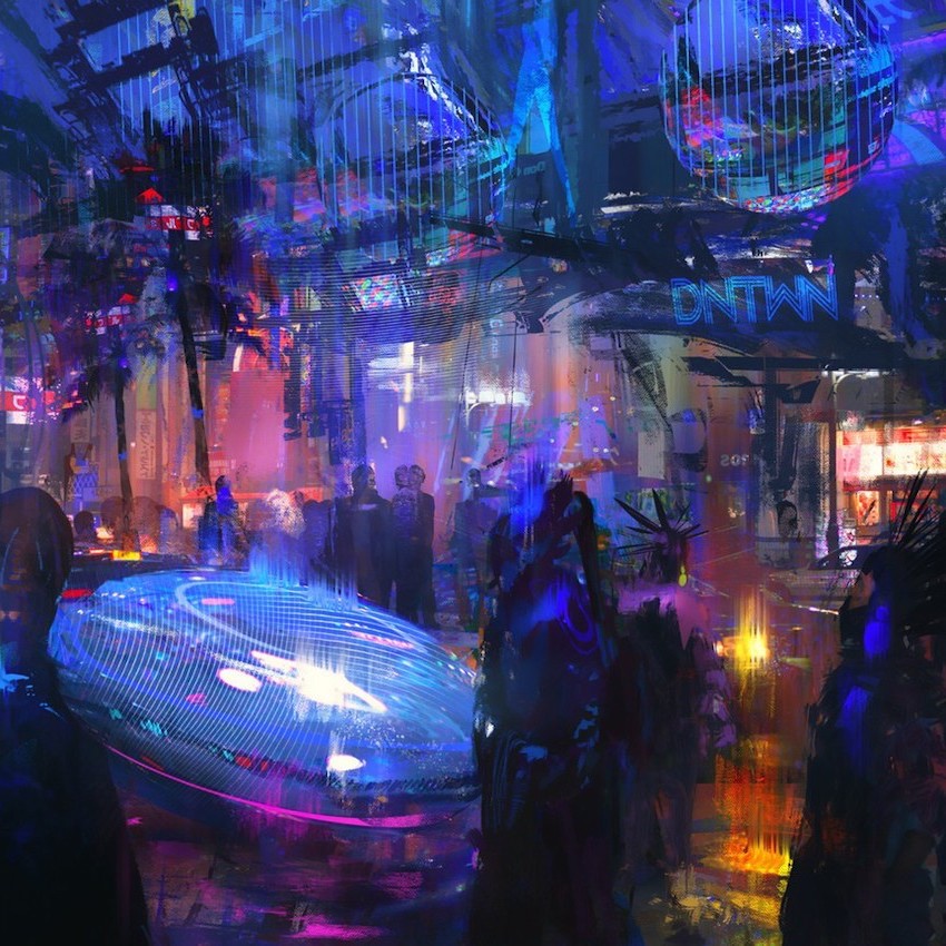
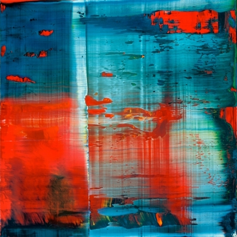
In this section we explore the capabilities of this CNN by running some experiments. In the previous section we recreated the trials by Gatys et al. and found that our CNN produces desirable results. Now, we synthetize some artworks by using additional content and style images. For content, we use a photo of the Berkeley Campanile, a Doge meme, and a drawing of Ash Ketchum. For style, we use some famous artworks and some random photos and an additional drawing.
First batch
 |
 Style |
 Style |
 Style |
 Style |
||||
|
Neckarfront |
Result |
 Result |
 Result |
||||
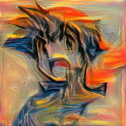
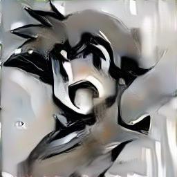
 Ash Ketchum |
 Result |
 Result |
 Result |
 Result |
||||
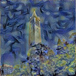
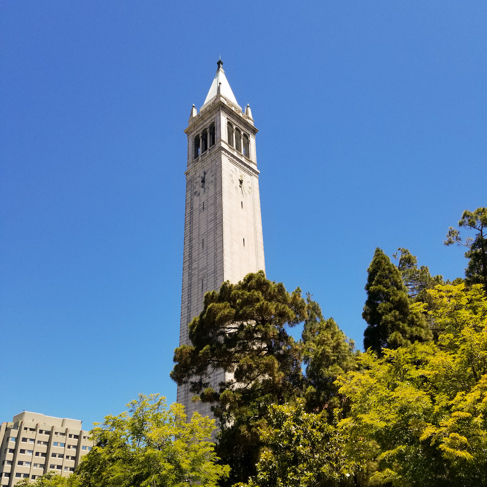 Berkeley Campanile |
 Result |
 Result |
 Result |
 Result |
||||
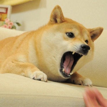 Doge |
 Result |
 Result |
 Result |
 Result |
Second batch
|
|
 Style |
 Style |
 Style |
 Style |
||||
|
Neckarfront |
 Result |
 Result |
 Result |
||||
|
Ash Ketchum |
 Result |
 Result |
 Result |
 Result |
||||
|
Berkeley Campanile |
 Result |
 Result |
 Result |
 Result |
||||
|
Doge |
 Result |
 Result |
 Result |
 Result |
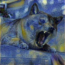
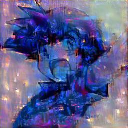
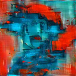
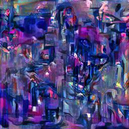
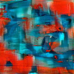
Observations
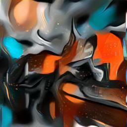
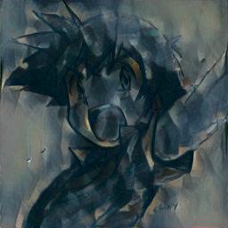
Depending on the style image, the resulting artwork is more or less abstract. We noticed that the more well-defined edges, ripples, or corners a style image has, the more details the resulting image will contain. Note, for example, the random pictures used does not contain prominent sharp edges, so the resulting images are smoother and more abstract. Yet, the color feel and overall style is properly transferred.
Errors & Final Thoughts
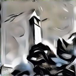
Failed art synthesis
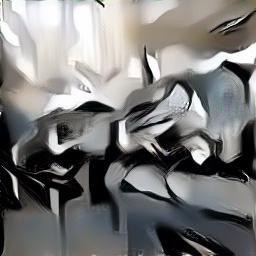
We encountered some examples where the image stylization did not work well. In the images below we have some example where the style image seems to be superposed on top of the content image (although after a careful look it is actually a generated texture resembling the style image), and in other the style surpasses the content. We believe the this could have happened either because the ratio α/β was not set properly (there was more weight on the style rather than the content) or because the epoch number was too small. Here we present some failed examples.
|
|
 Style |
 Style |
||
|
Ash Ketchum |
 Result |
 Result |
||
|
Doge |
 Result |
 Result |
Conclusion
In this project, we have demonstrated that convolutional neural networks are not just exceptionally efficient for pattern recognition, but they are powerful on inference and image synthesis. Although CNNs are not yet capable of generating original artworks autonomously (that is, without explicit human help), they can do an excellent job on copycatting they style of current works of art. Ultimately, creativity is a really hard thing to artificially simulate, but the creativeness of people is unlimited, and maybe one day it may become a reality.