
Overview
Background
Artificial Intelligence (AI) has been experiencing an enormous growth in recent years as it is becoming a major area of research in both neuroscience and computer science fields. Deep Learning, an algorithmic extension from Machine Learning and AI, is enabling computers to automatically learn and infer information from experience without being explicitly programmed how to do so. We will briefly explore Convolutional Neural Networks (CNNs or ConvNets), which are a class of deep neural networks commonly used to analyze visual imagery. CNNs provide with an exciting and powerful tool to recognize underlying patterns or features in a set of images through a process that mimics the way the human brain operates. Convolutional Neural Networks are being used ubiquitously to solve a wide variety of learning problems involving recognition and classification tasks. In this project we will design and implement a CNN that will help us to detect facial keypoints in images.
Architecture of a Convolutional Neural Network
Convolutional Neural Networks (CNNs), like standard neural networks, are made up of “neurons” with learnable weights and biases that are obtained during a complex process of training. In the case of image recognition, images are represented as numeric matrices which are sent through a series of convolutional layers, pools, and fully connected layers where each node (or neuron) uses an activation function to compute the output of that node given an input or set of inputs. Each neural network learns its weights and biases in a process called Back propagation, which refers to the process of fine-tuning the weights of a CNN based on the error rate (i.e. loss) obtained in the previous epoch (i.e. iteration). Proper tuning of the weights ensures lower error rates, making the model reliable by increasing its generalization. In addition, the optimization function (“Adam” in our example) will help us find the weights that will, hopefully, yield a smaller loss in the next iteration. “Adam” is an optimization algorithm that can be used instead of the classical stochastic gradient descent procedure to update network weights iterative based the training data.
 The CNN consist of two main sections: the convolutional learning layers and the classification layer. |
A CNN generally consists of the following components:
Input layer it represents the input for the neural network to processed. In our CNN we take a grayscale (single channel) image as input. The dimensions of the image range from 80x60 for part 1 and 240x180 for part 2. The pixel values range from 0 to 255, but these values are usually normalized to improve the model performance.
Convolution layer: it consists of a group of stacked matrices (channels) that are obtained through a convolution operation between the previous layer and a set of small matrix filters known as kernels. Each new channel represents the convolution outcome for every applied Kernel. A visualization of the convolution process is shown below.
 This convolution only takes into account the existing values of the input matrix. (towardsdatascience.com) |
 This convolution includes a padding that extends beyond the dimension (mirror) of the input matrix. |
Activation function: it is non-linear function applied to the weighted sum of the inputs of a neuron in any neural network. It determines whether that neuron should be activated or not. The activation function was inspired by the biological propagation of signals happening in human neurons in the brain. Below is a comparison between a biological neuron and an artificial one.
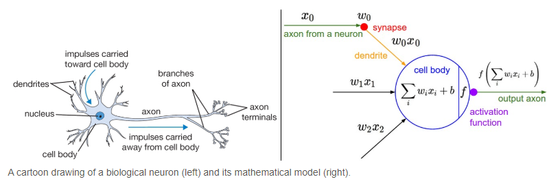 The activation function simulates the signal generated by a biological neuron which is then sent through an axon (neural edge in the case of the artificial version) |
Two common examples of activation function are the sigmoid function and ReLU (Rectified Linear Unit). ReLU is one of the most used activation functions since it is computationally efficient and allows neural networks to converge significantly fast. On top of that it is quite simple and allows backpropagation! It is expressed as max(0,x) which means that any input below 0 is set to 0 while any positive input is allowed to pass as it is.
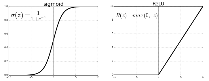 These functions are non-linear. Note: ReLU stands for Rectified Linear Unit. |
Pooling layer: it is a filter whose job is to downsample the data coming out from a convolutional layer. The filter is very simple: a fix-sized matrix “box” that sweeps over the input matrices and computes a value by condensing all the numbers inside its boundaries. For this project we will use a Maxpool layer, which selects the maximum value lying within the region covered by the filter. An animated example is shown below where the Maxpool filter size is 3.
 In this example the Maxpool filter is of size 3x3. (towardsdatascience.com) |
Fully connected layers: they connect every neuron in one layer to every neuron in another layer. In principle, they are the same as the traditional multi-layer perceptron neural network (MLP) where a flattened matrix goes through a fully connected layer to compute a prediction. Fully Connected Networks (FCN) are well known as the workhorses of deep learning and they are used in a wide variety of applications. In this project, it will help us to detect facial keypoints, also known as landmarks, which generally specify the areas of the nose, eyes, mouth, and face outline. The input for our FCN will be a flattened version of last CNN layer and the output will be a one-dimensional list of keypoints coordinates. Below a classic FCN is shown.
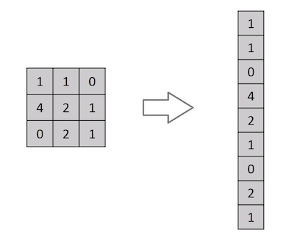 The Fully Connected Network takes a one-dimensional array of values and outputs a one-dimensional array of values as well. |
 A standard Fully Connected Network, also known as a multi-layer perceptron neural network (MLP). |
PART 1: Nose tip detection
Implementing the DataLoader
For the first part, we use the IMM Face Database for training small model whose goal is detecting lower part of the nose tip (the philtrum). The dataset has 240 facial images of 40 persons and each person has 6 facial images in different viewpoints. The dataset includes annotation for all images and each file contains 58 facial keypoints. We dive up the first 32 persons (192 images) as the training set and the remaining 8 persons (48 images) as the validation set. Before designing our CNN, we need to implement a dataloader to iterate over the image set. For this part of the project, the dataloader retrieves the images and their corresponding keypoints (landmarks), resize the image into a smaller size (80x60), and normalize the pixels from 0-255 into 0-1. It also converts the matrix representation of the image into a Pytorch tensor. Here are some raw examples provided by the dataloader.
 Randomly transformed face. |
 Randomly transformed face. |
 Randomly transformed face. |
 Randomly transformed face. |
Designing the CNN model
Now that we have the dataloader, we design a convolutional neural network using the Pytorch CC Module. The architecture for this simple CNN consists of three convolutional layers with 12, 16, and 32 channels respectively, kernel size of 3x3, three maxpool layers of size 2x2, two fully connected layers with output size of 120 and 2 respectively. Each convolutional layer and the first FC layer are followed by a ReLU operation. The detailed model is shown below.
ConvNetNose(
  (conv1): Conv2d(1, 12, kernel_size=(3, 3), stride=(1, 1))
  (pool1): MaxPool2d(kernel_size=2, stride=2, padding=0, dilation=1, ceil_mode=False)
  (conv2): Conv2d(12, 16, kernel_size=(3, 3), stride=(1, 1))
  (pool2): MaxPool2d(kernel_size=2, stride=2, padding=0, dilation=1, ceil_mode=False)
  (conv3): Conv2d(16, 32, kernel_size=(3, 3), stride=(1, 1))
  (pool3): MaxPool2d(kernel_size=2, stride=2, padding=0, dilation=1, ceil_mode=False)
  (fc1): Linear(in_features=1280, out_features=120, bias=True)
  (fc2): Linear(in_features=120, out_features=2, bias=True)
)
Optimization and training
We use the Mean Squared Error (MSE) loss function (torch.nn.MSELoss) and the Adam (torch.optim.Adam) optimizer to train the neural network using a learning rate of 1e-3. Training the model for at least 17 epochs can reduce the validation error significantly. The train and validation losses during each epoch are shown in the following plot.
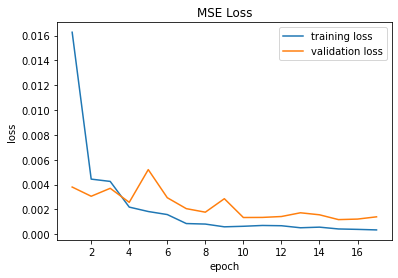 Mean Squared Error (MSE) for the nose tip CNN. |
As we can see, MSE loss steadily decreases on every epoch despite finding some spikes along the way. The MSE loss was different on different training runs but the overall losses remained within similar ranges.
Results
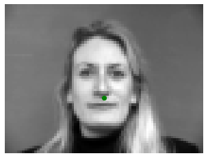
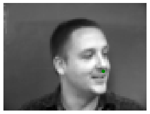
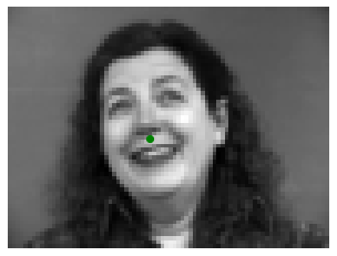
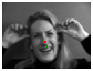
fter the CNN model is properly trained, we test it by feeding some input images. Since the dataloader provides with randomly transformed images we can test the model several times. The results after the training are shown below where the green points are the ground-truth annotation and the red points are the predictions.
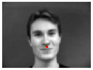 Randomly transformed face with correctly detected nose tip keypoint (landmark). |
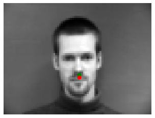 Randomly transformed face with correctly detected nose tip keypoint (landmark). |
 Randomly transformed face with correctly detected nose tip keypoint (landmark). |
 Randomly transformed face with correctly detected nose tip keypoint (landmark). |
|||
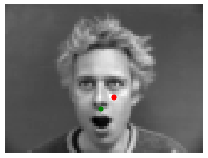 Randomly transformed face with incorrectly detected nose tip keypoint (landmark). |
 Randomly transformed face with incorrectly detected nose tip keypoint (landmark). |
 Randomly transformed face with incorrectly detected nose tip keypoint (landmark). |
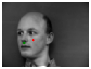 Randomly transformed face with incorrectly detected nose tip keypoint (landmark). |
Although the majority of test images were annotated pretty good there were some faces that were with unsatisfactory detections. This is probably due to various reasons such as the randomness of the dataloader (some images could have been rotated too much), the lightning in the original image (some faces have one side of the face lit), exaggerated facial expressions, hair style, or even hands on the air. Overall, our CNN does its job at approximating the location of the nose tip. Next, we not only predict a single point, but all 58 facial keypoints.
PART 2: Full Facial Keypoints Detection
Implementing the DataLoader
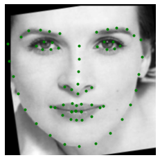
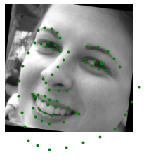
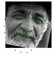
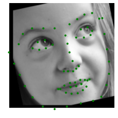
The data loader job for this part of the project is similar to the previous one, but this time it applies additional transformation to decrease the chances of overfitting. The transformations to be applied are the following: resizing images to 240x180, randomly rotating both images and keypoints between -15 and 15 degrees, randomly shifting both images and keypoints in both vertical and horizontal directions by 5%, and finally randomly changing the contrast and brightness by 15% and 10% respectively. This process is known as inline data augmentation since we are generating more new images from the existing ones on the fly. We show sampled images from the dataloader visualized with ground-truth keypoints below.
 Randomly transformed face. |
 Randomly transformed face. |
 Randomly transformed face. |
 Randomly transformed face. |
Designing the CNN model
The architecture for this CNN is a bit more complex than the previous one to account for the increased image size and keypoints. This time the model consists of five convolutional layers (8, 14, 20, 27, and 35 channels respectively), four maxpool layers (2x2), and three fully connected layers (512, 256, 116) and a ReLU operation on every layer except the last one. The detailed architecture is shown below.
ConvNetFace(
  (conv1): Conv2d(1, 8, kernel_size=(7, 7), stride=(1, 1))
  (pool1): MaxPool2d(kernel_size=2, stride=2, padding=0, dilation=1, ceil_mode=False)
  (conv2): Conv2d(8, 14, kernel_size=(5, 5), stride=(1, 1))
  (pool2): MaxPool2d(kernel_size=2, stride=2, padding=0, dilation=1, ceil_mode=False)
  (conv3): Conv2d(14, 20, kernel_size=(3, 3), stride=(1, 1))
  (pool3): MaxPool2d(kernel_size=2, stride=2, padding=0, dilation=1, ceil_mode=False)
  (conv4): Conv2d(20, 27, kernel_size=(5, 5), stride=(1, 1))
  (pool4): MaxPool2d(kernel_size=2, stride=2, padding=0, dilation=1, ceil_mode=False)
  (conv5): Conv2d(27, 35, kernel_size=(3, 3), stride=(1, 1))
  (fc1): Linear(in_features=1575, out_features=512, bias=True)
  (fc2): Linear(in_features=512, out_features=256, bias=True)
  (fc3): Linear(in_features=256, out_features=116, bias=True)
)
This time we also present a CNN Diagram for our model:
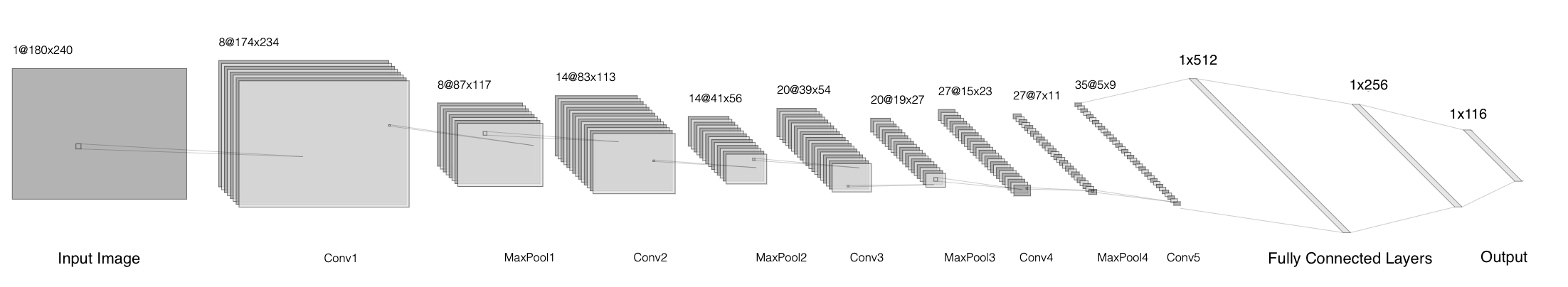 CNN Diagram for our keypoint (landmark) detection model. |
Optimization and training
In a similar way to the previous net, we use the Mean Squared Error (MSE) loss function and the Adam optimizer to train this CNN with the following hyperparameters: learning rate of 1e-3 and 30 epochs. The train and validation losses during each epoch are shown in the following plot.
 Mean Squared Error (MSE) for the facial keypoint CNN. |
Once again, the MSE loss varied on every training run but it stayed within a similar range.
Results
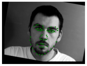
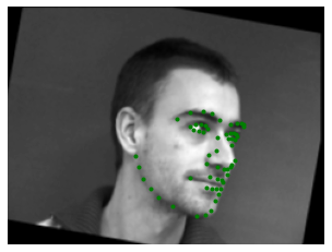
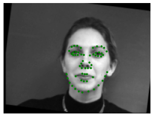
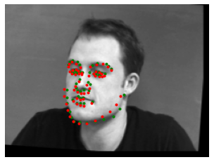
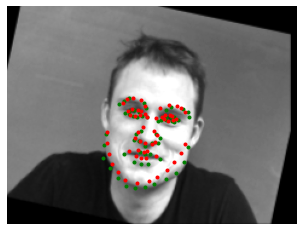
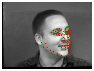
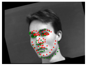
Finally, the results after the training are shown below where the green points are the ground-truth annotation and the red points are the CNN predictions.
 Randomly transformed face with correctly detected facial keypoints (landmarks). |
 Randomly transformed face with correctly detected facial keypoints (landmarks). |
 Randomly transformed face with correctly detected facial keypoints (landmarks). |
 Randomly transformed face with correctly detected facial keypoints (landmarks). |
|||
 Randomly transformed face with incorrectly detected facial keypoints (landmarks). |
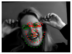 Randomly transformed face with incorrectly detected facial keypoints (landmarks). |
 Randomly transformed face with incorrectly detected facial keypoints (landmarks). |
 Randomly transformed face with incorrectly detected facial keypoints (landmarks). |
This time the results were varied. Considering the small size of our CNN (which was designed this way to produce faster results in an average laptop), it was not surprising to see more inaccurate keypoint detections. The reasons for this accuracy are likely to be the same as with the nose tip CNN: excessive rotation, facial expressions, overall illumination (brightness & contrast). Despite its small size and relatively small dataset, our CNN manages to get great approximations. Next, we will explore how to use a standard CNN model to boot prediction accuracy. The learned kernel filters for the first two convolutional layers are displayed below
 Each image represents a learned kernel of size 7x7. They started with random values |
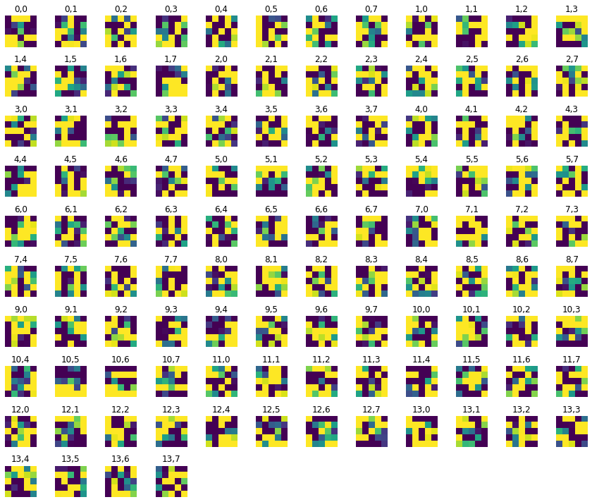 Each image represents a learned kernel of size 5x5. They started with random values. |
Part 3: Train With Larger Dataset
Overview
In this final part of the project we will go a step further and will use a standard CNN model such as ResNet (residual neural network) to improve our predictions even more. We will also use a larger image dataset (6666 annotated images) and will use Google Colab's deep learning environment to have access to significantly more computational resources. Just as a side note, a ResNet, is based on pyramidal cells found in the cerebral cortex. In order to simulate this, residual neural networks skip connections, or create shortcuts to jump over some layers (Wikipedia).
Implementing the DataLoader
For this part, we use a larger face dataset containing 6666 images of varying image sizes, and each image has 68 annotated facial keypoints. In addition, we are provided with bounding boxes (left, top, width, height) for the face that become helpful during training, as we need to crop the image and feed only the face portion to the model. We resize the cropped image into 224x224 and apply the same data augmentation from part 2. The dataset is split into two subsets: training (6000 images) and validation (666 images). Below we show some images sampled from our new dataloader along ground-truth landmarks.
 Annotated facial keypoints. |
 Annotated facial keypoints. |
 Annotated facial keypoints. |
 Annotated facial keypoints. |
 Annotated facial keypoints. |
Designing the CNN model
This time we use ResNet-18, a standard convolutional neural network that is 18 layers deep. Deeper neural networks such as ResNet-18 are more difficult to train due the significant increase of filters, weights and biases to be learned. We use Pytorch’s resnet18 model to save us some time during the design. Before we can use it, we need to make two modifications on this model: For the first convolutional layer, you need to change the input channel to 1 for as the inputs are grayscale images. For the last fully connected layer, the output channel number should be 68 * 2 = 136, which represents the (x, y) coordinates of the 68 landmarks for each face. This adjustment process is known as neural network finetuning. The resulting model is shown below.
ResNet(
  (conv1): Conv2d(1, 64, kernel_size=(7, 7), stride=(2, 2), padding=(3, 3), bias=False)
  (bn1): BatchNorm2d(64, eps=1e-05, momentum=0.1, affine=True, track_running_stats=True)
  (relu): ReLU(inplace=True)
  (maxpool): MaxPool2d(kernel_size=3, stride=2, padding=1, dilation=1, ceil_mode=False)
  (layer1): Sequential(
    (0): BasicBlock(
      (conv1): Conv2d(64, 64, kernel_size=(3, 3), stride=(1, 1), padding=(1, 1), bias=False)
      (bn1): BatchNorm2d(64, eps=1e-05, momentum=0.1, affine=True, track_running_stats=True)
      (relu): ReLU(inplace=True)
      (conv2): Conv2d(64, 64, kernel_size=(3, 3), stride=(1, 1), padding=(1, 1), bias=False)
      (bn2): BatchNorm2d(64, eps=1e-05, momentum=0.1, affine=True, track_running_stats=True)
    )
    (1): BasicBlock(
      (conv1): Conv2d(64, 64, kernel_size=(3, 3), stride=(1, 1), padding=(1, 1), bias=False)
      (bn1): BatchNorm2d(64, eps=1e-05, momentum=0.1, affine=True, track_running_stats=True)
      (relu): ReLU(inplace=True)
      (conv2): Conv2d(64, 64, kernel_size=(3, 3), stride=(1, 1), padding=(1, 1), bias=False)
      (bn2): BatchNorm2d(64, eps=1e-05, momentum=0.1, affine=True, track_running_stats=True)
    )
  )
  (layer2): Sequential(
    (0): BasicBlock(
      (conv1): Conv2d(64, 128, kernel_size=(3, 3), stride=(2, 2), padding=(1, 1), bias=False)
      (bn1): BatchNorm2d(128, eps=1e-05, momentum=0.1, affine=True, track_running_stats=True)
      (relu): ReLU(inplace=True)
      (conv2): Conv2d(128, 128, kernel_size=(3, 3), stride=(1, 1), padding=(1, 1), bias=False)
      (bn2): BatchNorm2d(128, eps=1e-05, momentum=0.1, affine=True, track_running_stats=True)
      (downsample): Sequential(
        (0): Conv2d(64, 128, kernel_size=(1, 1), stride=(2, 2), bias=False)
        (1): BatchNorm2d(128, eps=1e-05, momentum=0.1, affine=True, track_running_stats=True)
      )
    )
    (1): BasicBlock(
      (conv1): Conv2d(128, 128, kernel_size=(3, 3), stride=(1, 1), padding=(1, 1), bias=False)
      (bn1): BatchNorm2d(128, eps=1e-05, momentum=0.1, affine=True, track_running_stats=True)
      (relu): ReLU(inplace=True)
      (conv2): Conv2d(128, 128, kernel_size=(3, 3), stride=(1, 1), padding=(1, 1), bias=False)
      (bn2): BatchNorm2d(128, eps=1e-05, momentum=0.1, affine=True, track_running_stats=True)
    )
  )
  (layer3): Sequential(
    (0): BasicBlock(
      (conv1): Conv2d(128, 256, kernel_size=(3, 3), stride=(2, 2), padding=(1, 1), bias=False)
      (bn1): BatchNorm2d(256, eps=1e-05, momentum=0.1, affine=True, track_running_stats=True)
      (relu): ReLU(inplace=True)
      (conv2): Conv2d(256, 256, kernel_size=(3, 3), stride=(1, 1), padding=(1, 1), bias=False)
      (bn2): BatchNorm2d(256, eps=1e-05, momentum=0.1, affine=True, track_running_stats=True)
      (downsample): Sequential(
        (0): Conv2d(128, 256, kernel_size=(1, 1), stride=(2, 2), bias=False)
        (1): BatchNorm2d(256, eps=1e-05, momentum=0.1, affine=True, track_running_stats=True)
      )
    )
    (1): BasicBlock(
      (conv1): Conv2d(256, 256, kernel_size=(3, 3), stride=(1, 1), padding=(1, 1), bias=False)
      (bn1): BatchNorm2d(256, eps=1e-05, momentum=0.1, affine=True, track_running_stats=True)
      (relu): ReLU(inplace=True)
      (conv2): Conv2d(256, 256, kernel_size=(3, 3), stride=(1, 1), padding=(1, 1), bias=False)
      (bn2): BatchNorm2d(256, eps=1e-05, momentum=0.1, affine=True, track_running_stats=True)
    )
  )
  (layer4): Sequential(
    (0): BasicBlock(
      (conv1): Conv2d(256, 512, kernel_size=(3, 3), stride=(2, 2), padding=(1, 1), bias=False)
      (bn1): BatchNorm2d(512, eps=1e-05, momentum=0.1, affine=True, track_running_stats=True)
      (relu): ReLU(inplace=True)
      (conv2): Conv2d(512, 512, kernel_size=(3, 3), stride=(1, 1), padding=(1, 1), bias=False)
      (bn2): BatchNorm2d(512, eps=1e-05, momentum=0.1, affine=True, track_running_stats=True)
      (downsample): Sequential(
        (0): Conv2d(256, 512, kernel_size=(1, 1), stride=(2, 2), bias=False)
        (1): BatchNorm2d(512, eps=1e-05, momentum=0.1, affine=True, track_running_stats=True)
      )
    )
    (1): BasicBlock(
      (conv1): Conv2d(512, 512, kernel_size=(3, 3), stride=(1, 1), padding=(1, 1), bias=False)
      (bn1): BatchNorm2d(512, eps=1e-05, momentum=0.1, affine=True, track_running_stats=True)
      (relu): ReLU(inplace=True)
      (conv2): Conv2d(512, 512, kernel_size=(3, 3), stride=(1, 1), padding=(1, 1), bias=False)
      (bn2): BatchNorm2d(512, eps=1e-05, momentum=0.1, affine=True, track_running_stats=True)
    )
  )
  (avgpool): AdaptiveAvgPool2d(output_size=(1, 1))
  (fc): Linear(in_features=512, out_features=136, bias=True)
)
Optimization and training
Just as in the previous two parts of this project, we use the Mean Squared Error (MSE) loss function and the Adam optimizer to train this CNN with the following hyperparameters: learning rate of 1e-3, batch size of 1, but this time we only train 12 epochs in Google Colab to take advantage of GPU (graphics processing unit) acceleration. The train and validation losses during each epoch are shown in the plot below.
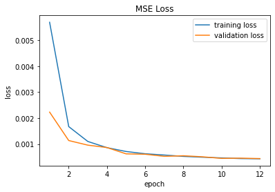 Mean Squared Error (MSE) for face landmarks. |
Results
We are provided with a set of 1008 images to try in our trained net. The test dataloader use the provided bounding boxes to crop and resize the face area of each image. Then each one is fed into our neural network to compute normalized landmarks which then are rescaled and relocated into their original dimensions. Some examples of our ResNet-18 landmark detections are shown below.
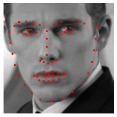 Landmarks detected in cropped image. |
 Landmarks detected in original image. |
 Landmarks detected in cropped image. |
 Landmarks detected in original image. |
 Landmarks detected in cropped image. |
 Landmarks detected in original image. |
 Landmarks detected in cropped image. |
 Landmarks detected in original image. |
 Landmarks detected in cropped image. |
 Landmarks detected in original image. |
Kaggle competition: We take the detected landmarks and save them into a csv file using the described formatting in the assignment specs and submitted to Kaggle for evaluation. The submission scored 10.01479, which is great considering only 12 training epochs!
Additional Results
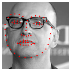
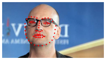
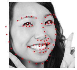
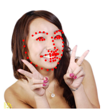
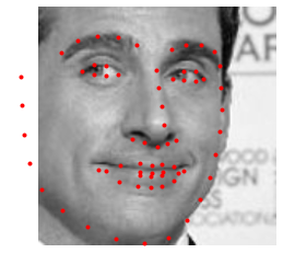
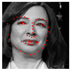
Finally, we try out some images from a custom photo collection. The landmark detection on portraits is pretty good. We also test some cartoon images just for fun to see how our trained net would perform. Popular anime characters have exaggerated features such as large eyes and small nose. The landmark detections on these samples were not perfect, but the model provided with reasonable approximations, nonetheless. It is worth mentioning that the training and validation dataset only include photographs.
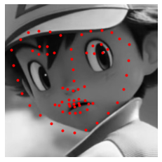 Landmarks detected in cropped image. |
 Landmarks detected in cropped image. |
 Landmarks detected in cropped image. |
 Landmarks detected in cropped image. |
 Landmarks detected in cropped image. |
 Landmarks detected in cropped image. |
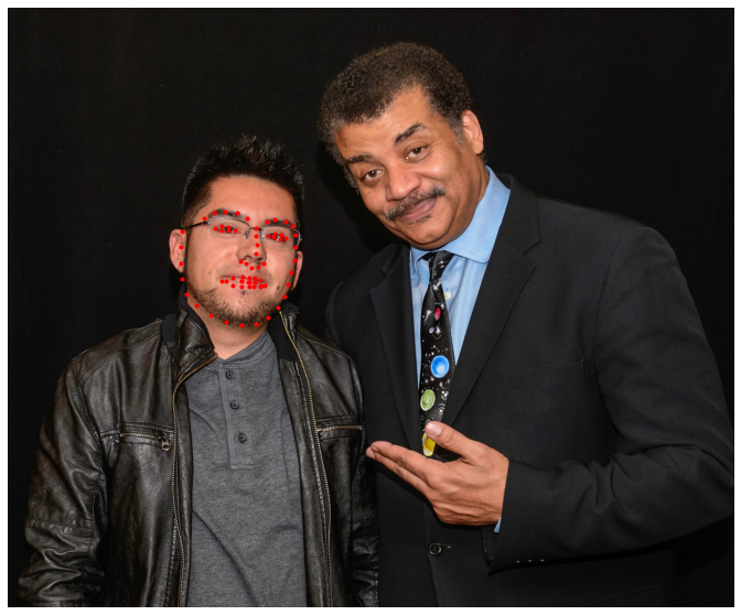 Landmarks detected in original image. |
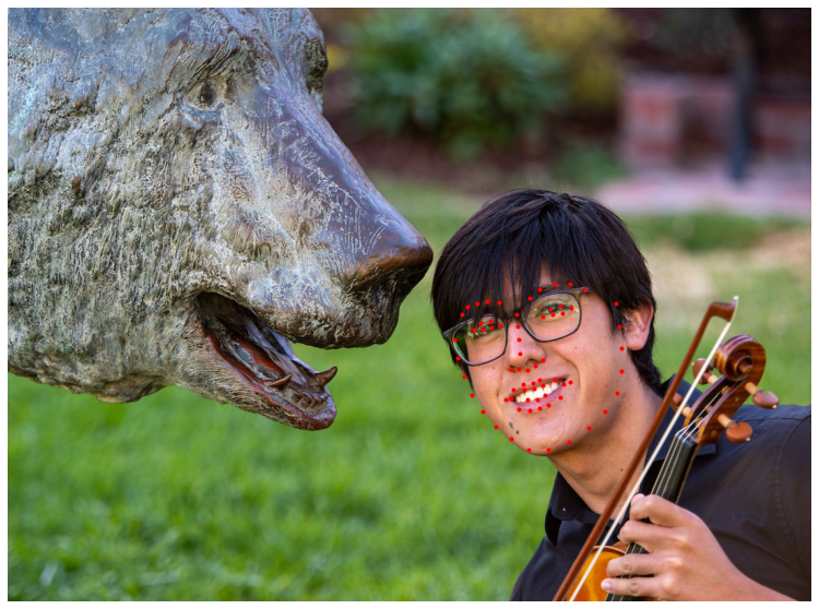 Landmarks detected in original image. |
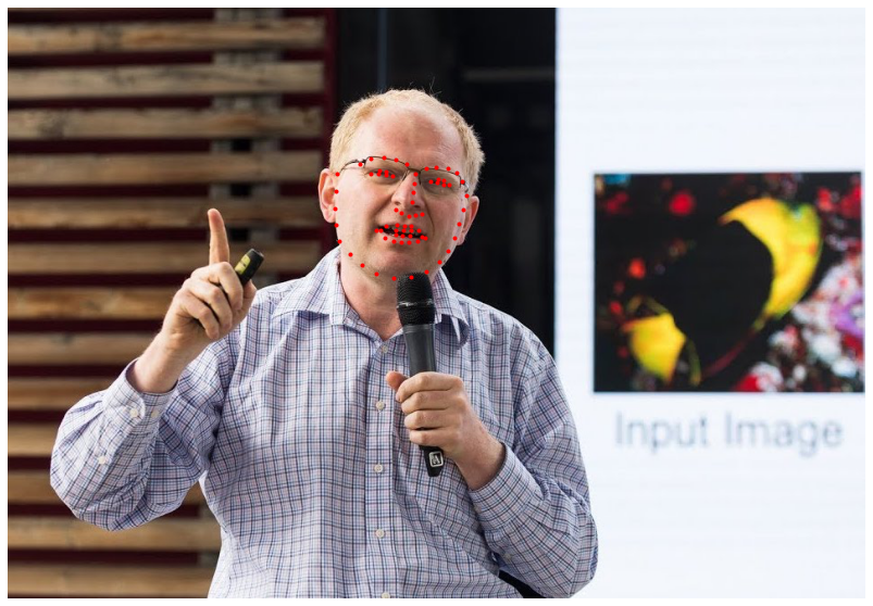 Landmarks detected in original image. |
 Landmarks detected in original image. |
 Landmarks detected in original image. |
 Landmarks detected in original image. |
Conclusion
In this project we explored the capabilities of deep learning using traditional convolutional neural networks (CNNs) and more robust varieties such as residual neural networks (ResNet-18). Facial keypoint detection is just one of the many cool and useful applications of Deep Learning. The possibilities of Machine Learning are boundless, and its power can sometimes be confused with pure magic!
References
Writing Custom Datasets, DataLoaders and Transforms:
https://pytorch.org/tutorials/beginner/data_loading_tutorial.html
Neural Networks Tutorial:
https://pytorch.org/tutorials/beginner/blitz/neural_networks_tutorial.html
A Comprehensive Guide to Convolutional Neural Networks:
https://towardsdatascience.com/a-comprehensive-guide-to-convolutional-neural-networks-the-eli5-way-3bd2b1164a53
Convolution Neural Networks vs Fully Connected Neural Networks:
https://medium.com/datadriveninvestor/convolution-neural-networks-vs-fully-connected-neural-networks-8171a6e86f15