Overview

In this project, we explore how we can create panoramas (image mosaics) from multiple images by registering, projective warping, resampling, and compositing them. The process to create panoramas can be reduced to computing homographies, which describes the projective geometry between two images angles (camera view) and a world plane. In other words, a homography maps image points which lie on a world plane from one view to another (a projection). The diagram below shows how we can project multiple view images into a single plane.

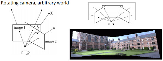Camera rotates when getting images

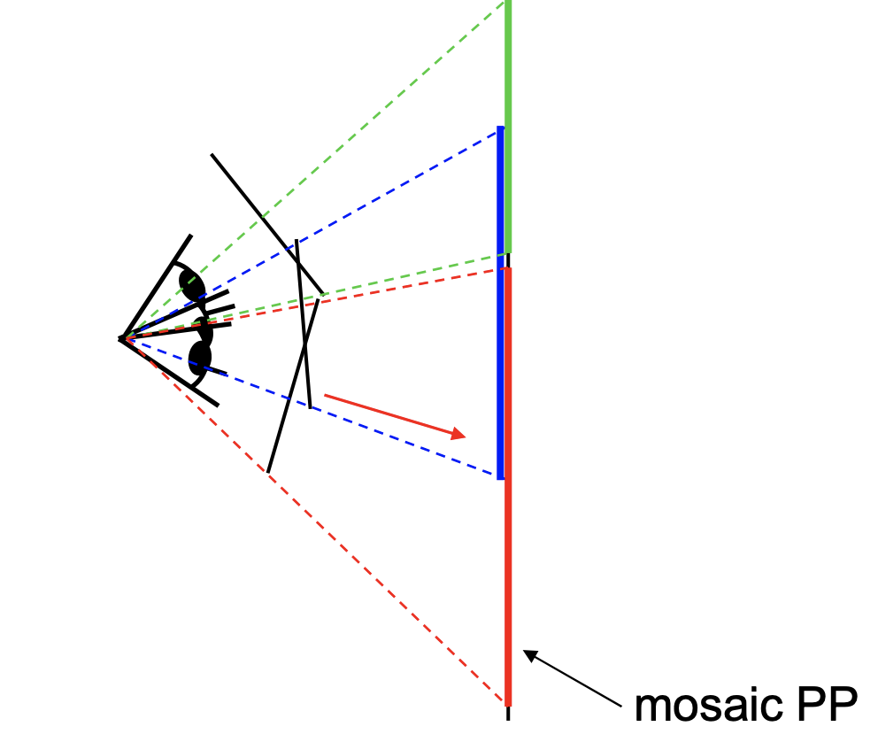Pencil or rays showing how rays projects onto each perspective view.

The project has been broken up into two parts. In Part A, we manually select the correspondence points from two images in order to compute the homography matrix. This matrix will then be used to rectify images and to compose a mosaic by stitching the two images. In Part B, we automate the stitching process by automatically selecting the correspondence points through the extraction of feature descriptors on each image and matching them between the two images. Finally, we use RANSAC to compute a homography matrix that can be used to produce the image mosaic.

PART A1: Getting the picture and points

Getting images

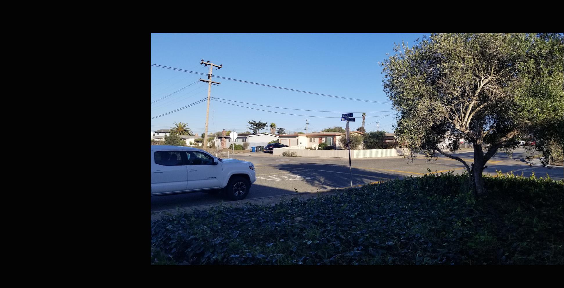
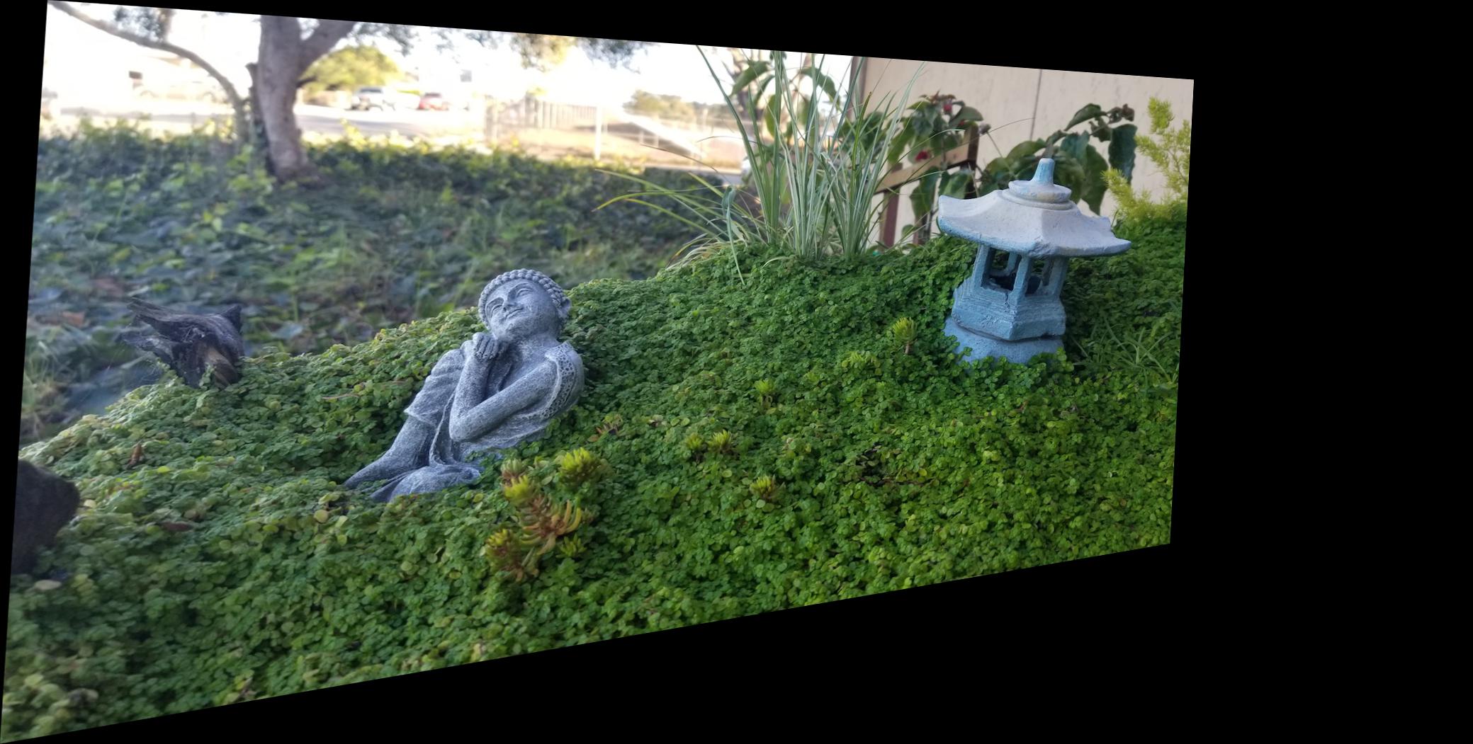
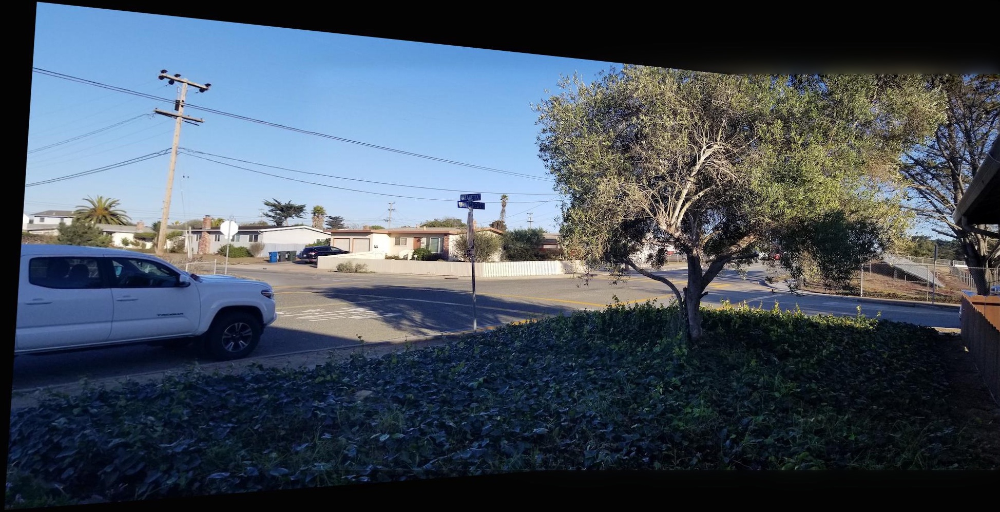
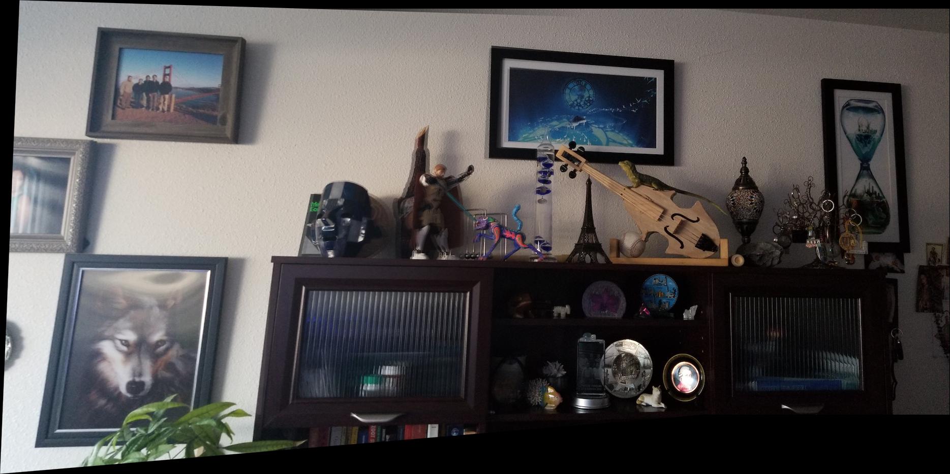
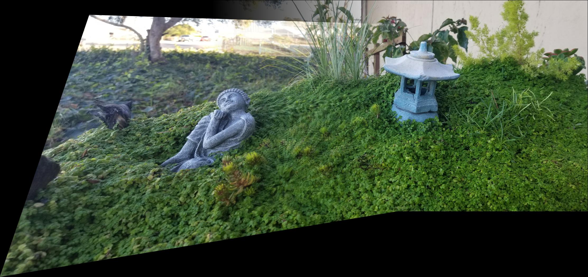
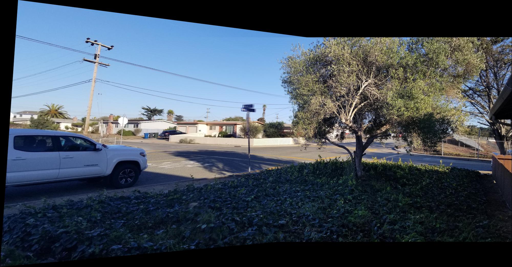
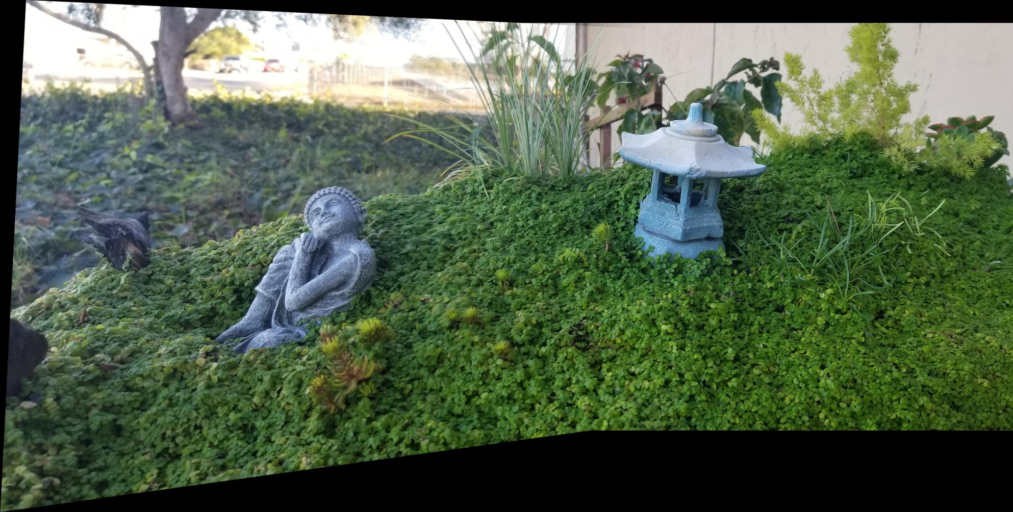
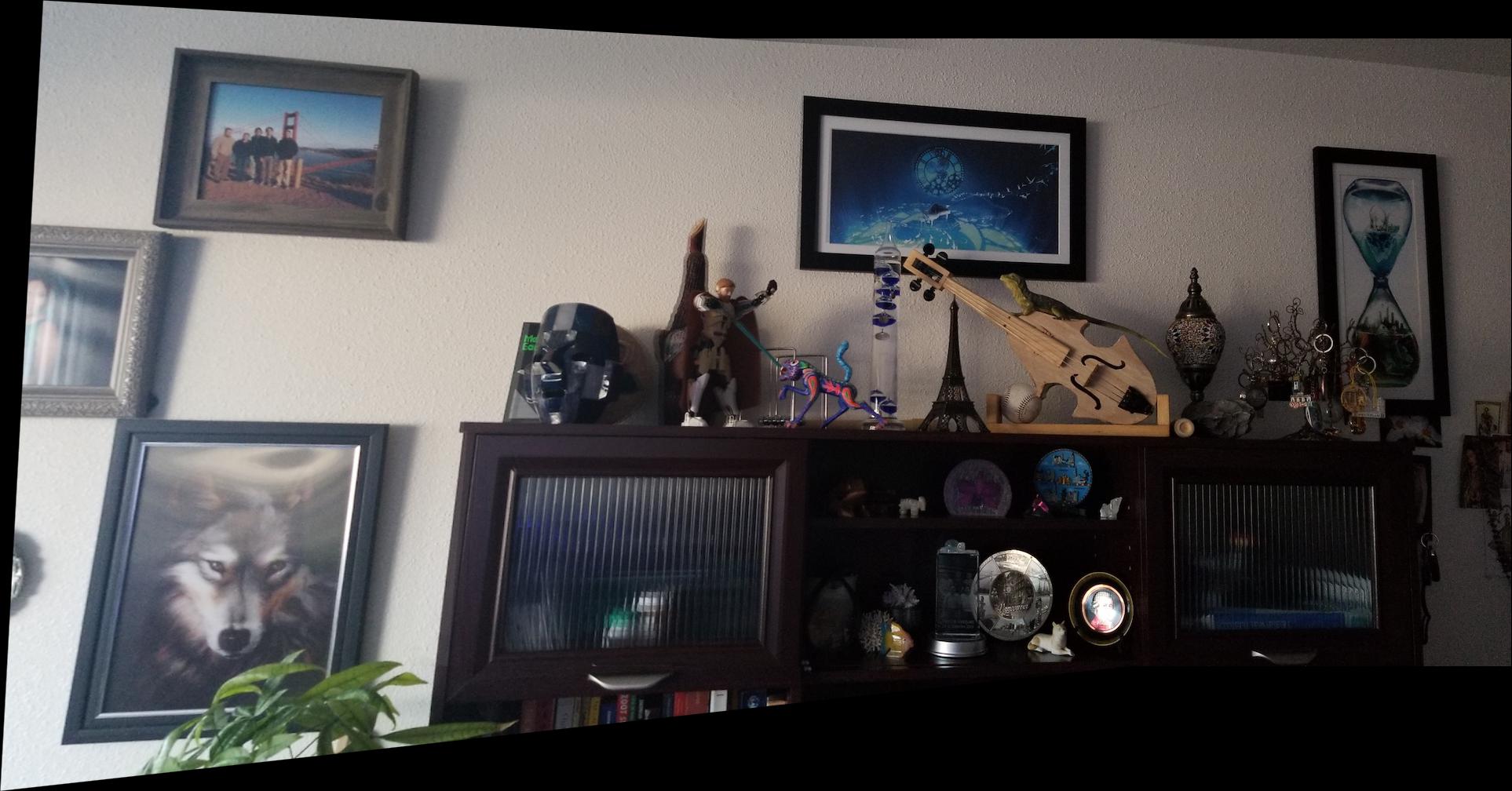
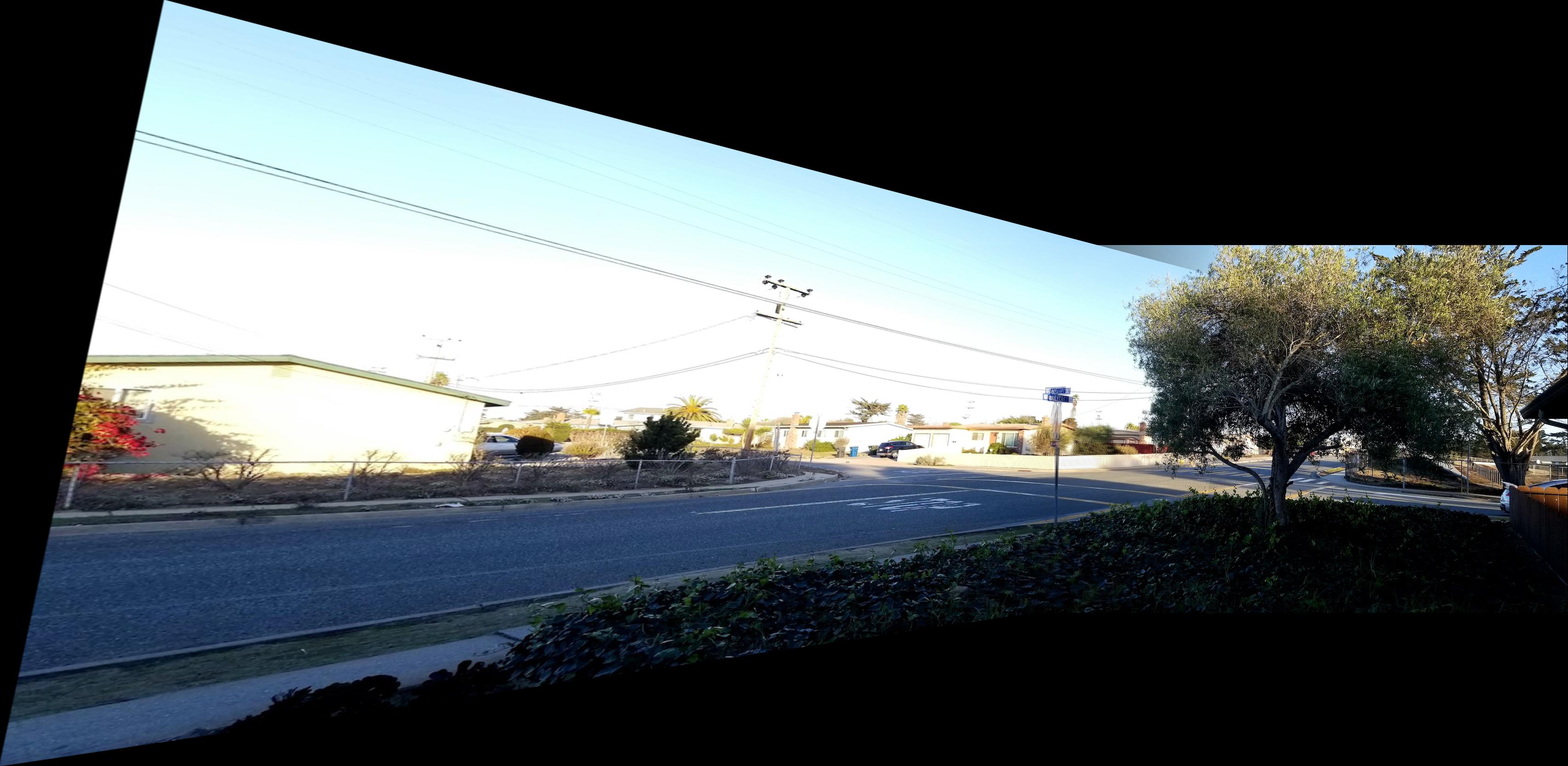
The first step was taking the pictures. In order to produce usable images, they have to be taking from the same point as if the camera is fixed in a standard tripod and it is only able to rotate. For this preliminary attempt, the pictures were taken by hand, making sure not producing noticeable movements sideways of back and forth. The resulting images are shown below.

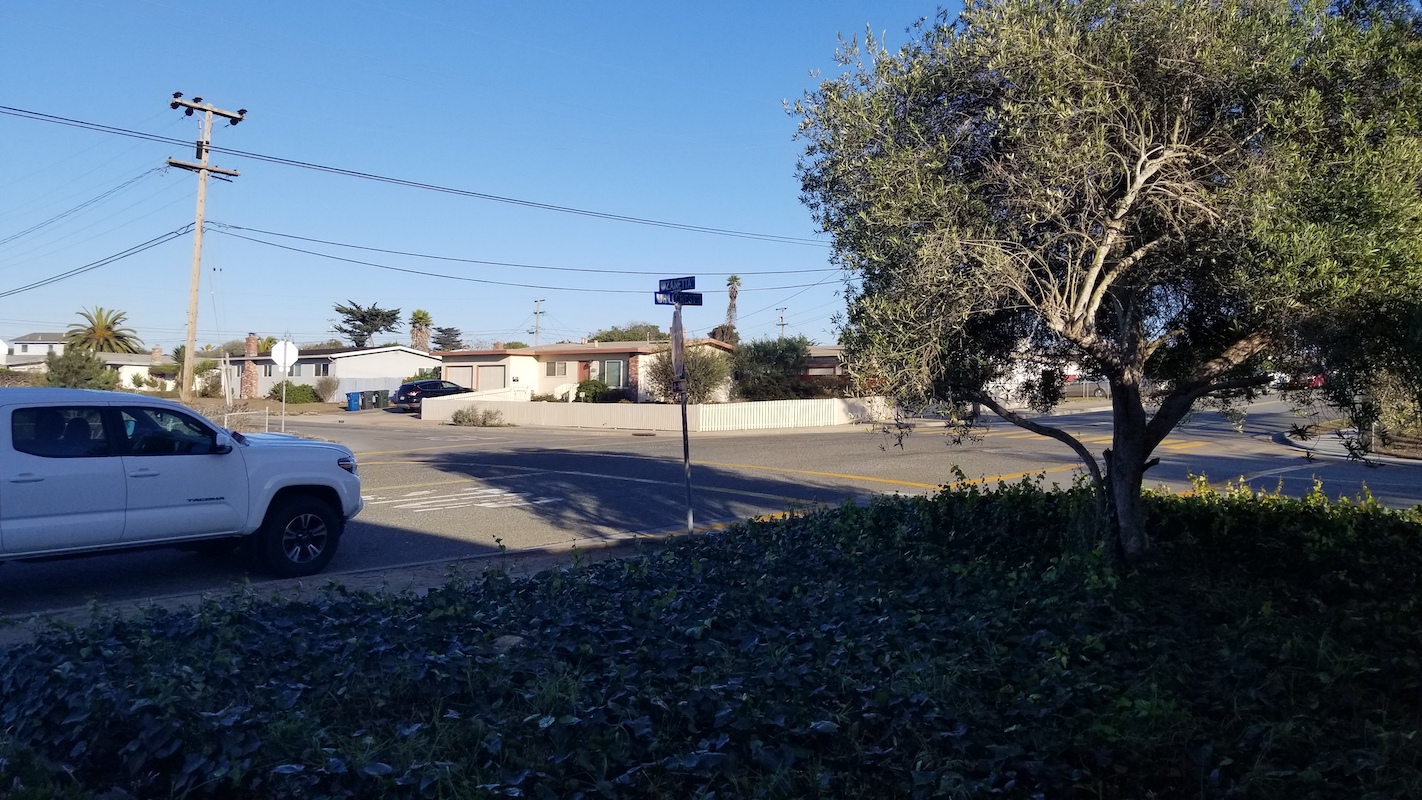Picture sample

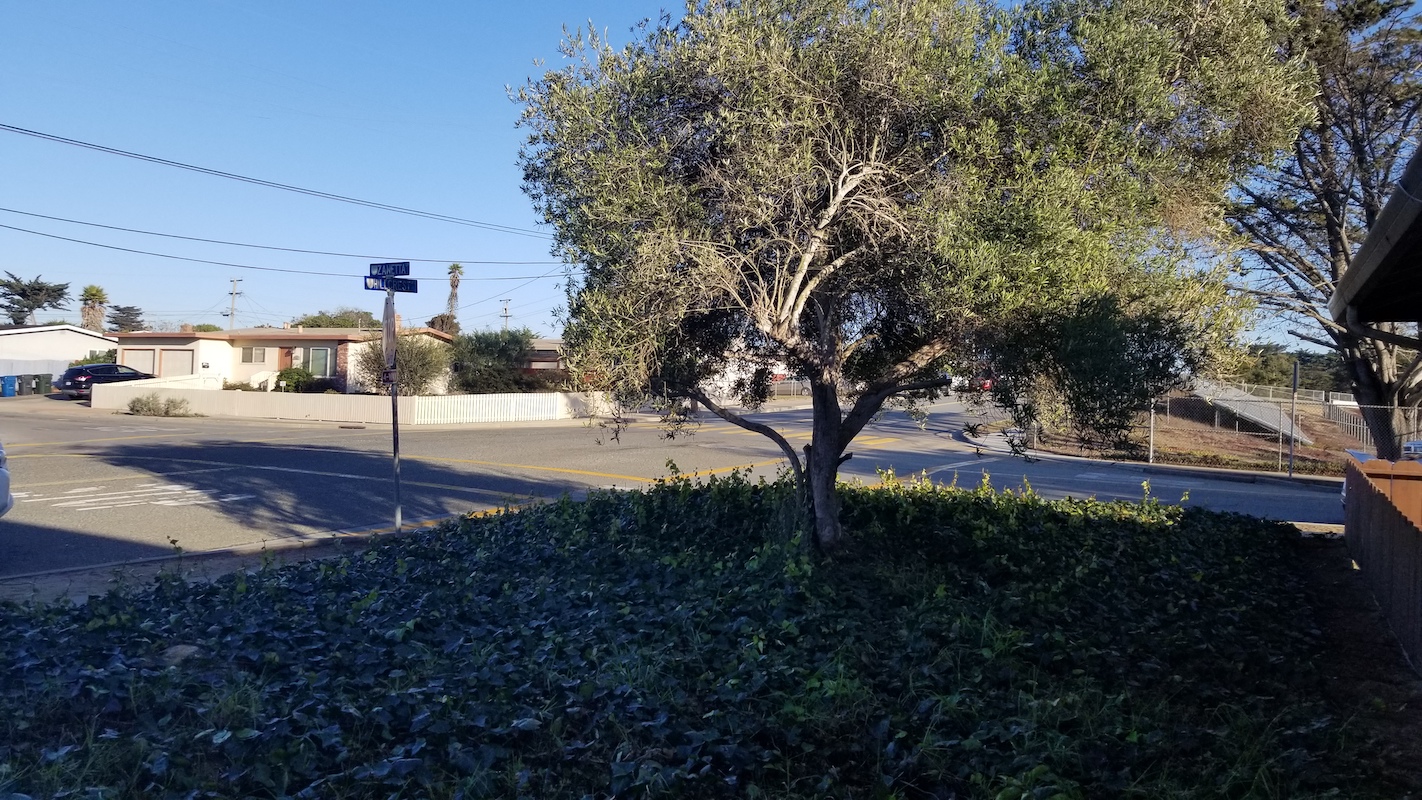Picture sample

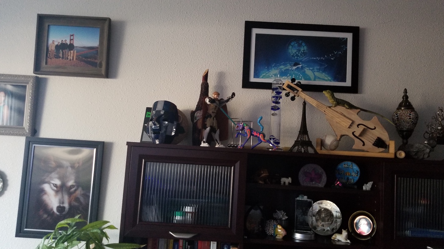Picture sample

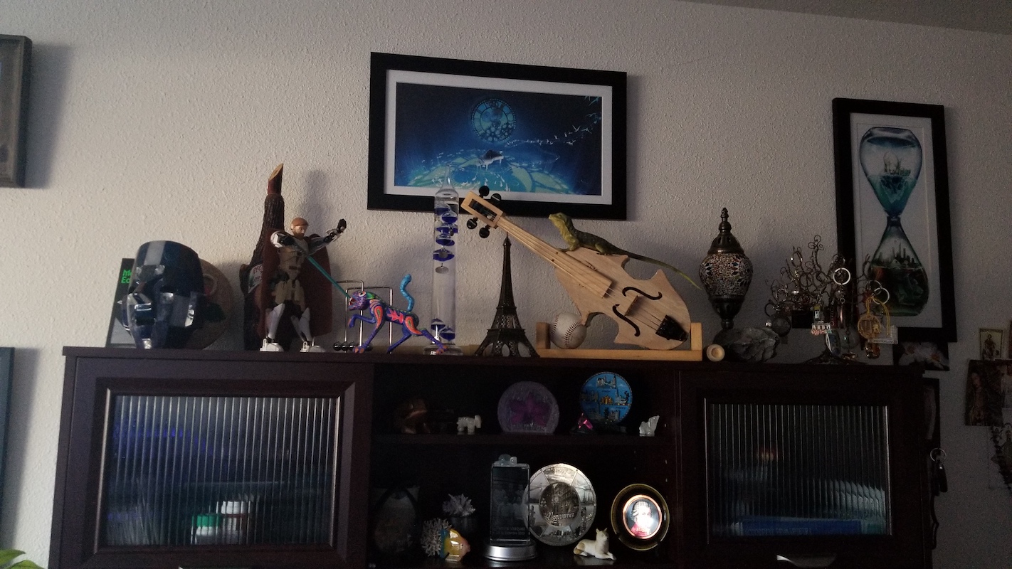Picture sample

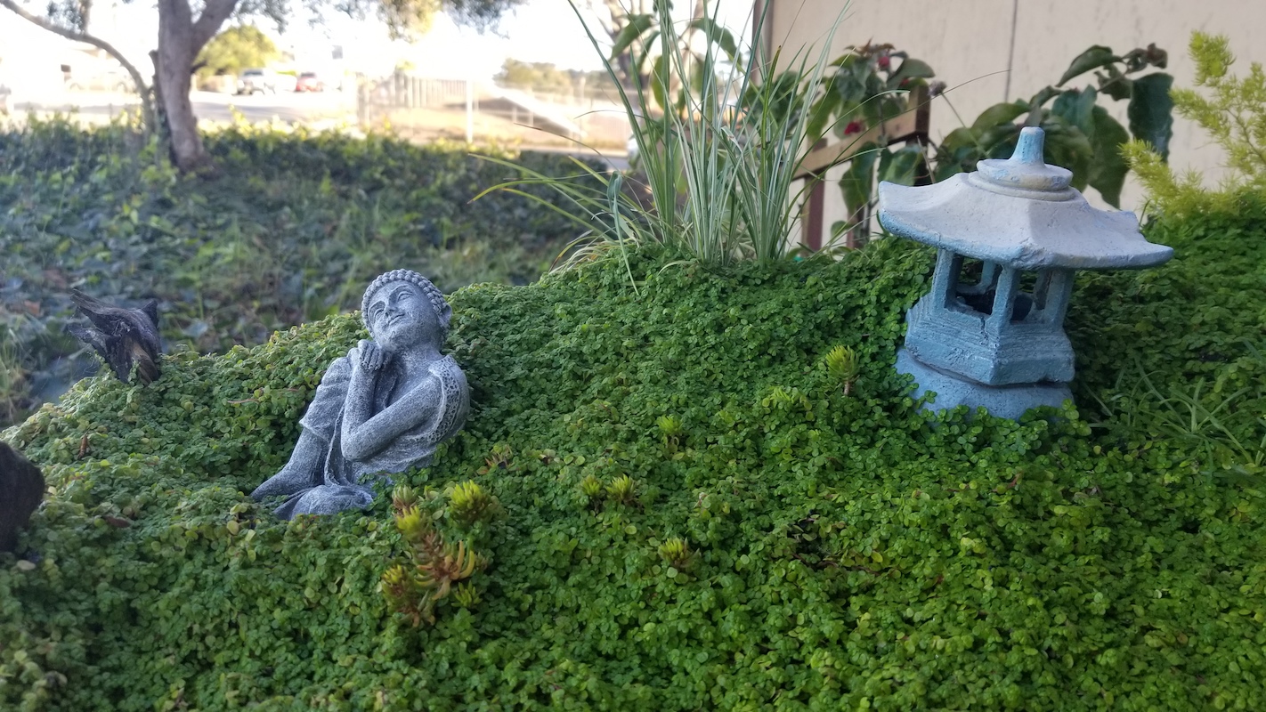Picture sample

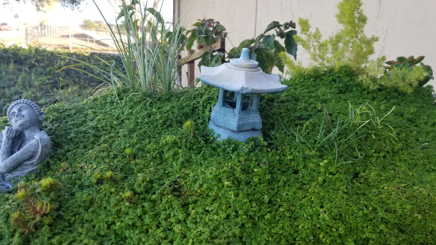Picture sample

Getting points

The next step is to define the correspondence pairs. For this, we created a small utility to manually select points and stored them into a file, this becomes handy during the development process of the project. When selecting point pairs, we need to make sure that the order in which the points are selected on each image must be the same, otherwise the homography matrix will be computed incorrectly. We place point in noticeable features such as tips and corners as shown below.

Picture sample

Picture sample

Warping

PART A2: Recovering Homographies

Setting up System of equations

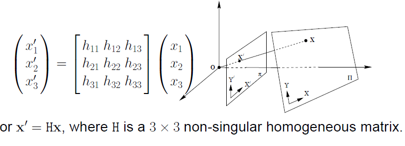
The homography (H for short) relates points in first image view to points in the second image view and since there are no constraints in either view. As previously pointed out, a homography is basically a projective transformation, whose matrix has 9 degrees of freedom. The following equation shown a basic setup where (x, y) and (x’, y’) are correspondence point located on each image.

Homography Matrix definition

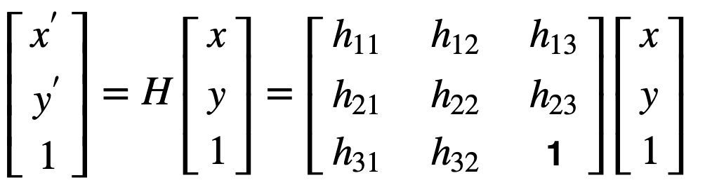
It is worth noticing that since we assume the photos to be taken from a fixed location (tripod) and similar settings (no zoomed in or out), we are not interested in scaling the image. Therefore, the element h33 is set to 1. Thus, this reduce out of degrees of freedom to 8, which will simply the computation by a bit.

Homography Matrix with one less degree of freedom

Setting up least squares problem

We now have 8 unknowns that need to be solved for. Upon arranging the system of equation in matrix form, we can model a model a least squares problem. Note that this problem cannot be solved analytically as the correspondence points does not necessarily match. Each pair of points can be represented as:

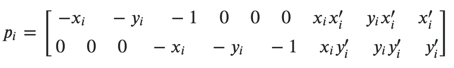Representation for a pair of points in least squares problem

So, stacking 8 pairs of points results in the following least square problem of the form 𝐴𝑥=𝑏, where the vector x represents the homography unknown elements.

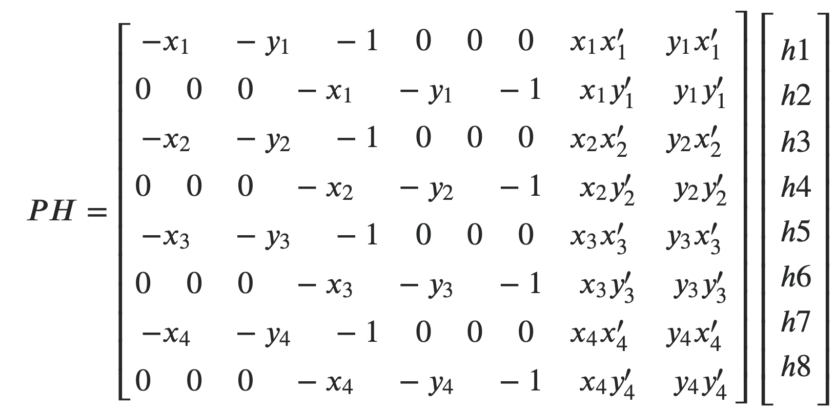Least squares matrix representation

After we have computed H, we are ready to start warping images!

PART A3: Image Warping

Computing bounding box (zero padding)

When we warp an image using the homography matrix H, it is possible that the transformed image extends beyond its original size. As a result, we can get a cropped warped image. To avoid this, we need to pad our original image to offset any possible canvas “overflow.” In order to compute the pad, first we forward warp the corners of the image to be warped to determine how large the output canvas need to be. For example, it is possible that one or more corner coordinates map negative coordinates in x and y or go beyond the dimension of the original image. To solve this, we compute x, y offsets so that the most negative coordinate in both x and y maps to zero. Also, any coordinates that goes beyond the height and width of the images is taken into account. Once these offsets are computed, they are applied to the images before warping, the resulting size if the image plus the padding is known as the bounding box. Note that the correspondence points must be offset as well, or preferably, a translation must be applied to the homography matrix to account for the offset. Below we show an example the forward-warped corners, and the padded image.

Forward warped corners. Note the negative coordines for some corners.

The size of the padded image is known as the bounding box.

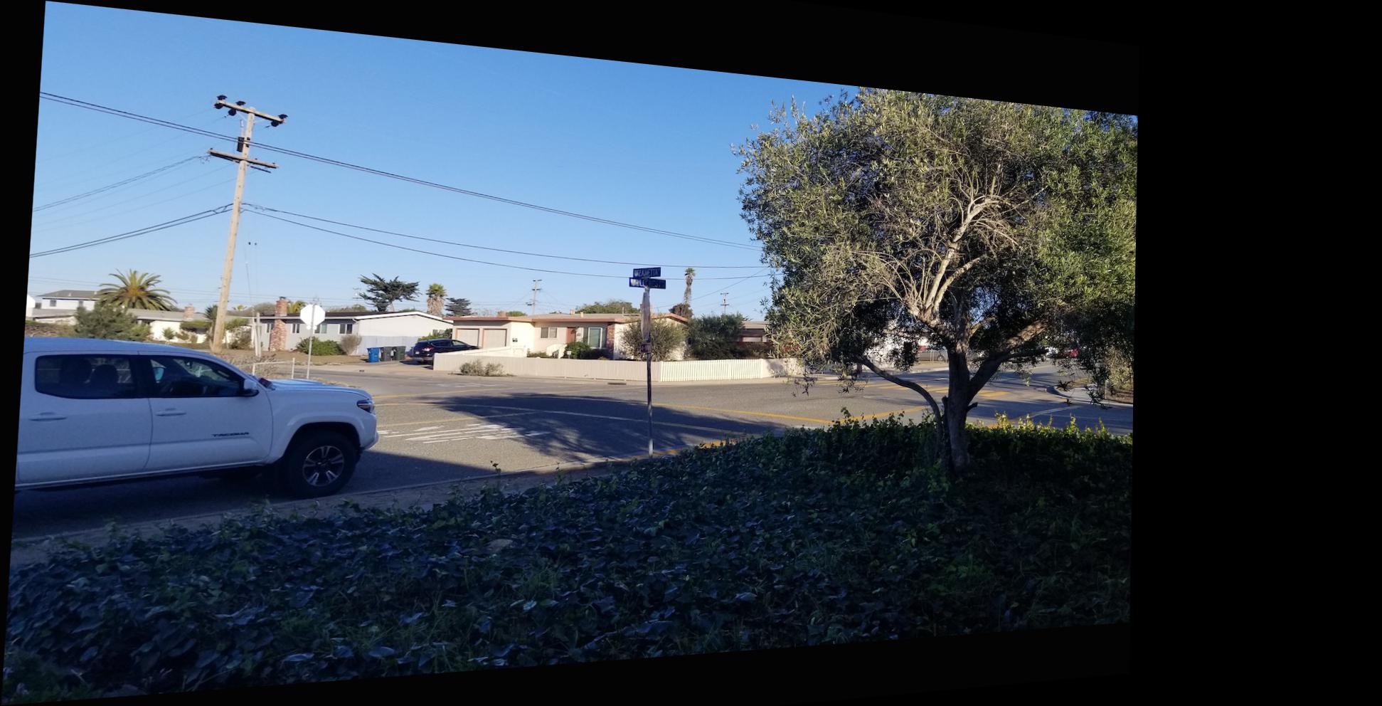
After the padding has been added to the image to be warped, we proceed by inverse warping the resulting canvas (aka. bounding box) coordinates to get the pixel values from the original image. We use linear interpolation to obtain pixel values on non-integer transformed coordinates. We decided to warp the left image onto the right image, so the following examples show the left image of every pair warped.

Picture sample

Warped image

Picture sample

Original

Image Rectification

PART A4: Frontal-parallel planar warp

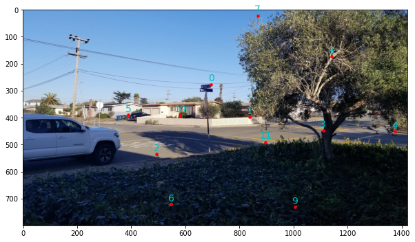
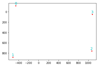
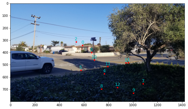
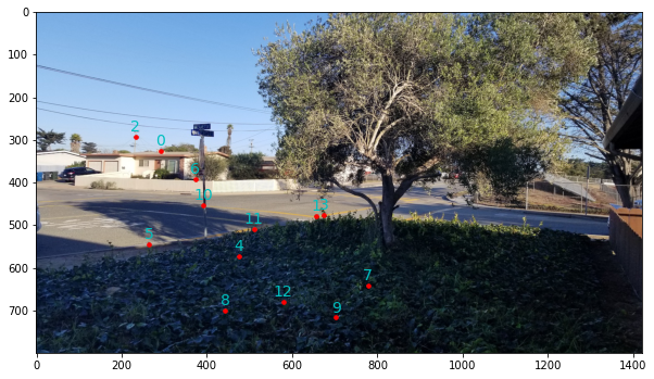
Now that the warping functions works, we can use it for a very useful application: rectifying images. Given a planar image taken in perspective, we can recover its frontal-parallel view by following the following steps: first, we select an image area that we want to be straightened by enclosing it with a sequence of points; second: we define the desired output shape for the selected image area, we do this by defining the ideal positions of the selected points, and third, we compute the homography matrix by using the set of correspondence points. For example, in the images below we the points 0 to 3 represent the selected area of the image, and the points from 4 to 7 represent our desired output shape for the selected area.

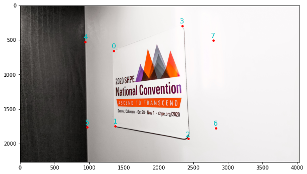Points 0-4: input area, 4-7: output shape.

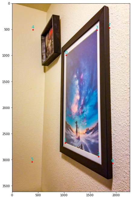Points 0-4: input area, 4-7: output shape.

Once the points are defined, we compute the homography matrix and warp the image into the desired shape. This application becomes handy when trying to pre-process text images so that it is easier for humans and computers to recognize the content. Some commercial scanning applications use this technique to improve scanning results.

Rectified image

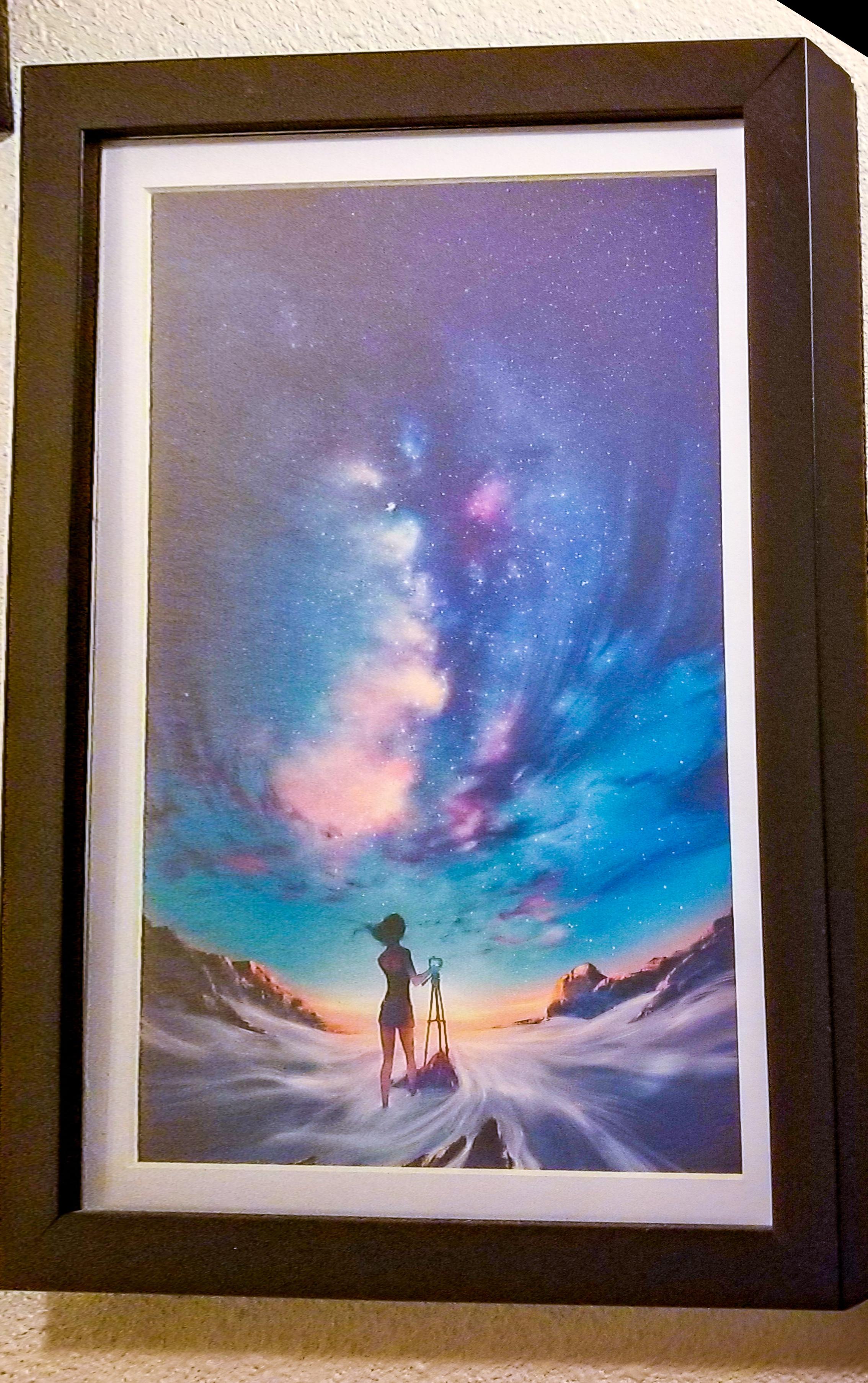Rectified image

Manual Stitching

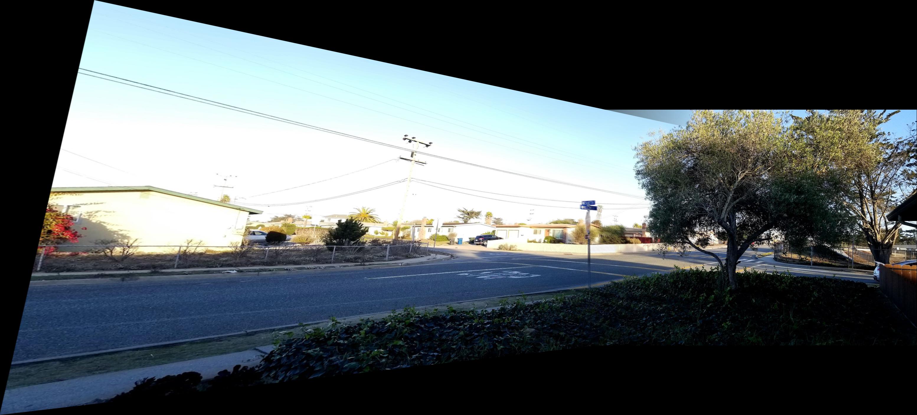
PART A5: Blending images into a mosaic

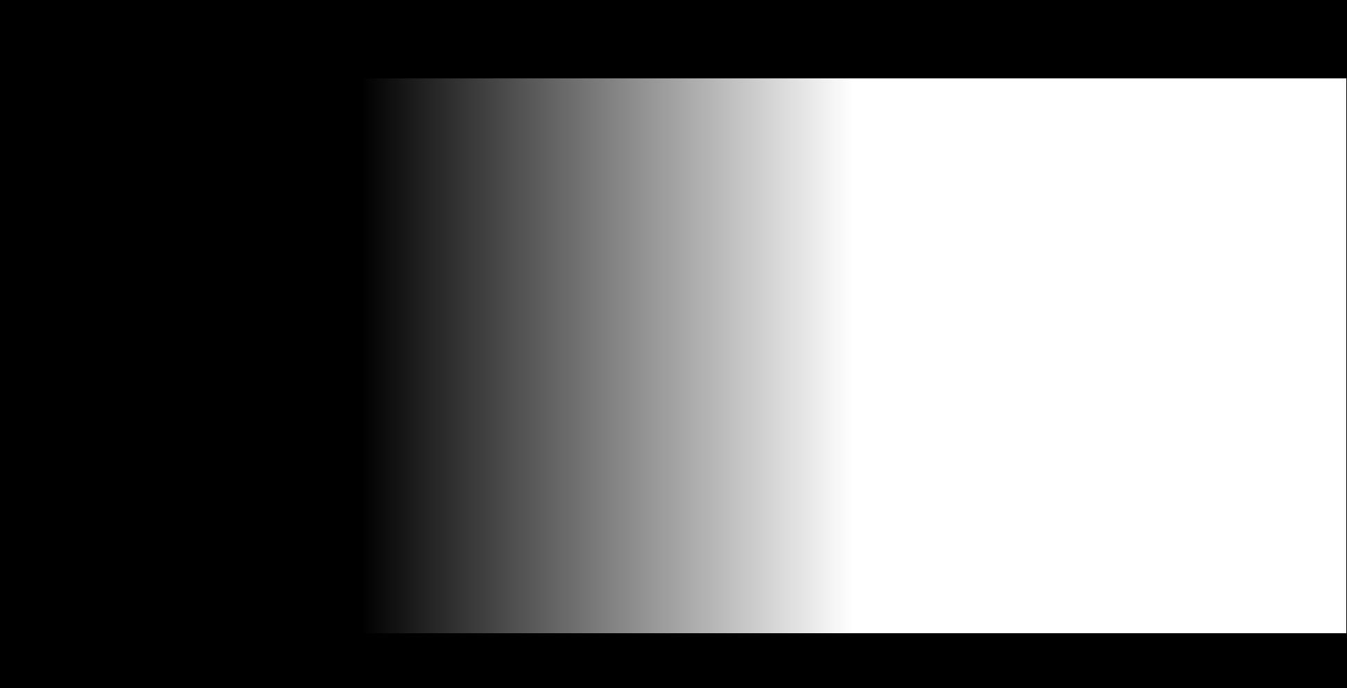
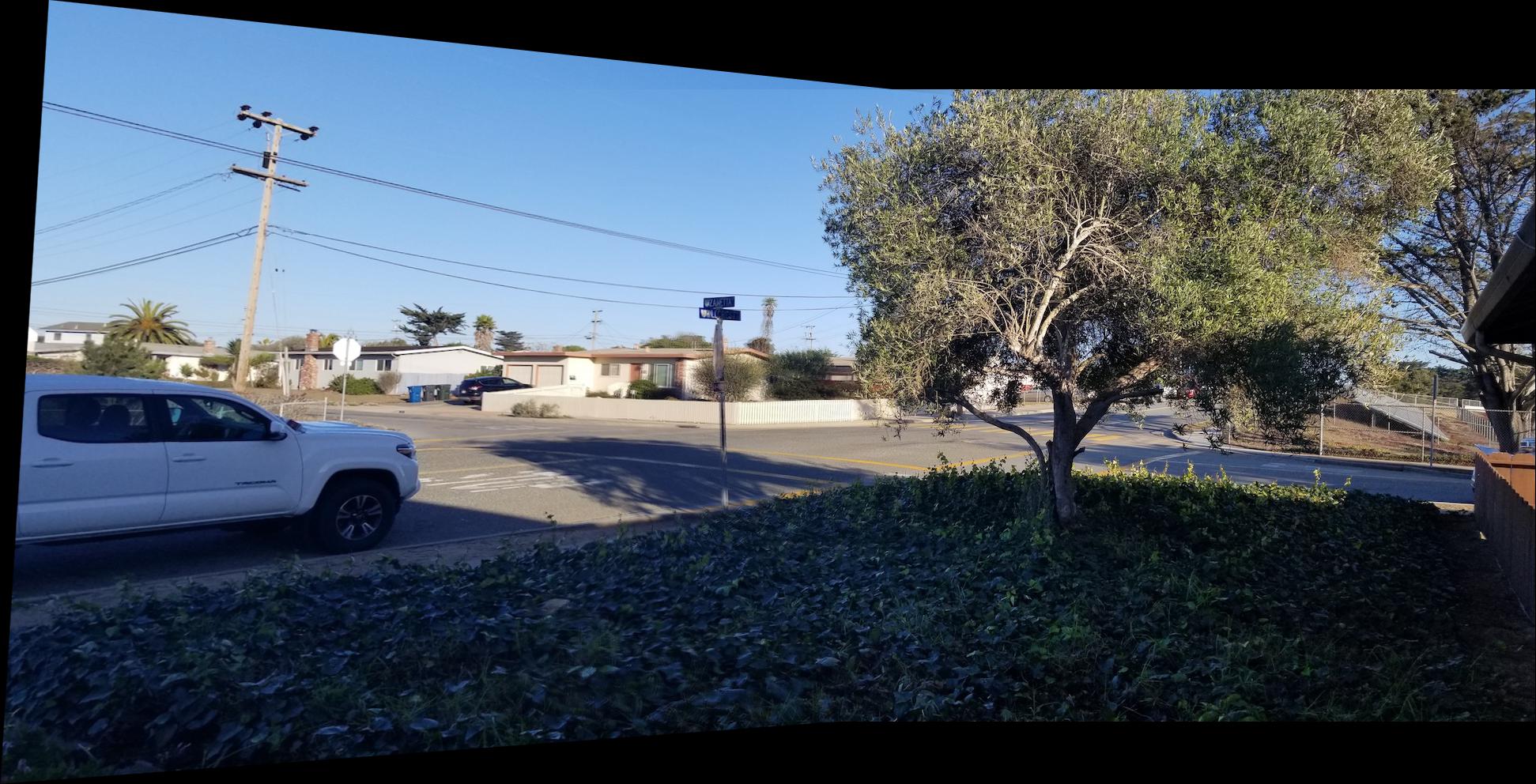
In order to compose a mosaic from our two images and manually selected points, we need to decide which image is going to be warped and which one will remain fixed. For this project, we decided to warp the left image onto the right one. Once we have warped the left image, we need to blend it to the right one. To do this we present three approaches where each of them has its advantages and disadvantages. The first approach was to use simple image superposition, that is, we just put the right image on top if the warped left image. This method is computationally cheap and fast, and it generates acceptable results as long as the alignment is well done, and the brightness does not vary between the two images. In the example below, we can see the edge of the image in the sky area of the image, but the alignment seems to be well done. The second approach consist in generating a gradient alpha mask for the fixed image (right one) so that it can be used to blend it with the left image using alpha crossfading (aka. weighted averaging). The resulting mosaic turns out to be a bit better in the sense that we don’t see the image edges, but there are some areas where we can see some ghosting. This method is pretty must as fast as the first one. Finally, we used to the multiresolution blending algorithm from project 2 to blend the warped left image, and padded fixed right image, and a mask for the fixed image to produce a smooth result. This approach is computationally more complex and expensive than the first two approaches. The result for each blending is shown below along some additional examples.

Mask

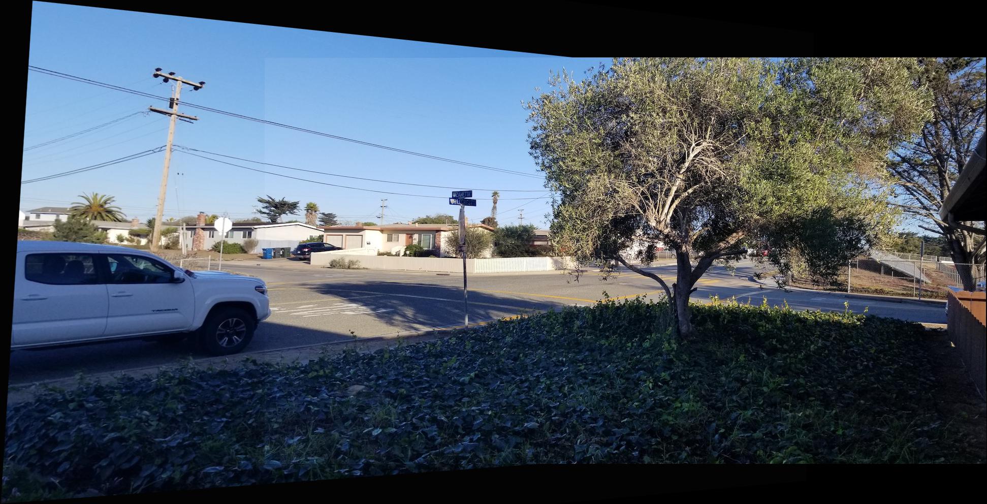Blended image

Mask

Blended image

Mask

Blended image

Additional examples blended with the gradient alpha mask.

Blended using Alpha crossfading blending (weighted averaging)

Blended using Alpha crossfading blending (weighted averaging)

Blended using Alpha crossfading blending (weighted averaging)

Feature Extraction & Matching

PART B1: Harris Interest Point Detector

In Part A, we manually selected correspondence points in the two images to compute our homography transformation matrix. In this part of the project, we are interested in automating the point selection process so that our stitching application is fully automatic as it should. We start by using the Harris Corner Detector, a corner detection operator that is frequently used in computer vision algorithms to extract corners and detect features of an image. In simple terms, a corner can be interpreted as the intersection of two edges, where an edge can be defined as a sudden change in brightness within a local image neighborhood. Corners are important features in an image, and they are generally called “interest points” which are invariant to translation, rotation and illumination.

Harris Corner Detector (datahacker.rs)

The Harris detector essentially finds the intensity difference for a displacement of (u,v) in all directions. Window function w(x,y) is either a rectangular window or gaussian window which gives weights to pixels underneath.

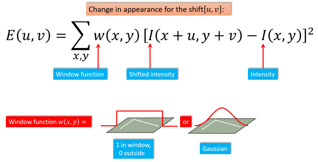Sum of squared differences (SSD) between these two patches

After we apply a Taylor expansion to equation below and using some mathematical steps (full derivation here, and here), we reach the following conclusion:

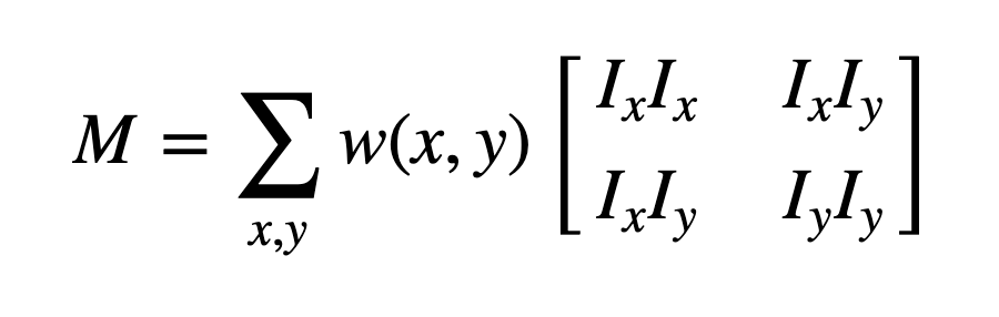Taylor expansion in matrix form.

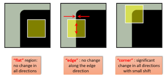
Where, I_x and I_y are image derivatives in x and y directions respectively. Finally, the score equation: R=det(M)−k(trace(M))² is derived from the equation above that is used to determine if a window can contain a corner or not. Note: det(M)=λ₁λ₂, trace(M)=λ₁+λ₂, and λ₁, λ₂ are the eigenvalues of M. Then the magnitudes of these eigenvalues decide whether a region is a corner, an edge, or flat.

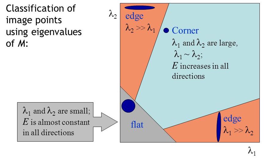Eigenvalues decide whether a region is a corner, an edge, or flat..

Finally, we apply the Harris detector to each image to be stitched to obtain a cloud of corners that will be used to find matching coordinates between them. We show the Harris corners overlaid on our selected left and right images.

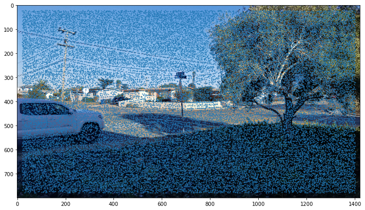Harris corners overlaid

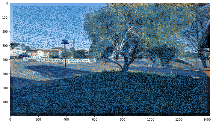Harris corners overlaid

PART B2: Adaptive Non-Maximal Suppression (ANMS)

Harris corner detector help us to detect possible feature candidates but there is a major problem: we have too many interesting points! Fortunately, Adaptive Non-Maximal Suppression (ANMS) is really useful for solving this problem. ANMS reduces the overall density by evenly selecting the interesting points across the image, thus only keeping the strongest features in each image region. The algorithm works by computing the suppression radius for each feature (strongest overall has radius of infinity), which is the smallest distance to another point that is significantly stronger (based on a robustness parameter c). ANMS can be summarized in the following steps:

1. Subtract current point coordinates from all others to compute relative coordinates to make the current point the origin.
2. Compute the L2-norm (Euclidean distance) between current point and all others.
3. Compute all strengths differences with current point’s strength based on the robustness parameter c = 0.9
4. Ignore all points whose strengths differences are non-positive, including the current one.
5. Find the nearest point with valid strength and store its distance in a fixed-size min heap.

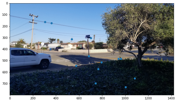
Note that the min heap will keep popping the minimum distance when it reaches capacity so that it will eventually hold the points with greatest radius. Also keep in minds that we aren't guaranteed to get the desired number features with the highest corner strengths, but instead, we get the most dominant points in each image region, which ensures we get spatially distributed strong points. The resulting Harris points are shown in the following images.

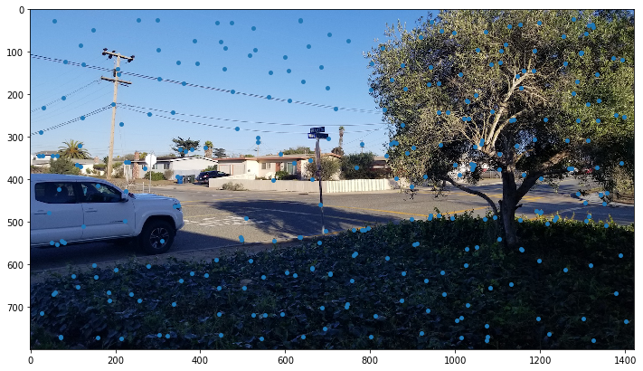ANMS point selection

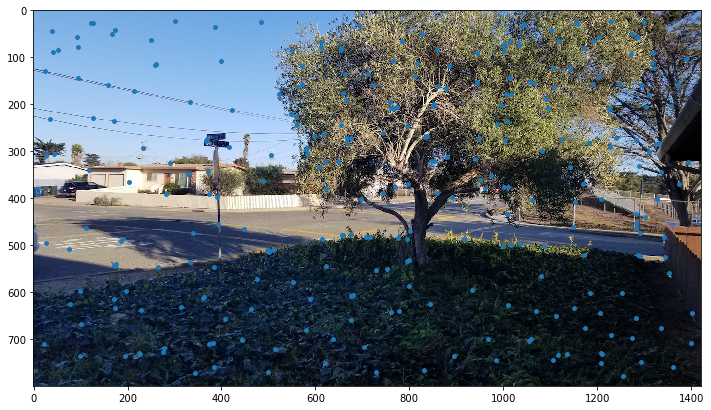ANMS point selection

PART B3: Feature Descriptor Extraction & Matching

Extracting Feature Descriptors

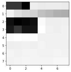
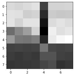
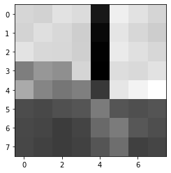
Now that we have a more manageable number of Harris points per image, we now ponder the problem of matching these points from one image to the other. One clever way to solve this is by extracting “Feature Descriptors,” that consist in getting a small image patch whose center is a Harris point. To create a feature descriptor, we take a Harris point’s (x, y) coordinate and extract an image area encompassing 20 pixels in every direction from the point (up, down, left, right). The resulting 41x41pixel patch is then downsized to an 8x8 pixel patch. The reason we take a larger patch and the resize it instead of just taking an 8x8 patch from the beginnings is that when we downsample the patch we create a nice blurred descriptor. In addition, after extracting these feature descriptors we normalized them so that their mean is 0 and their standard deviation is 1. This makes them invariant to affine changes in intensity in both bias and gain.

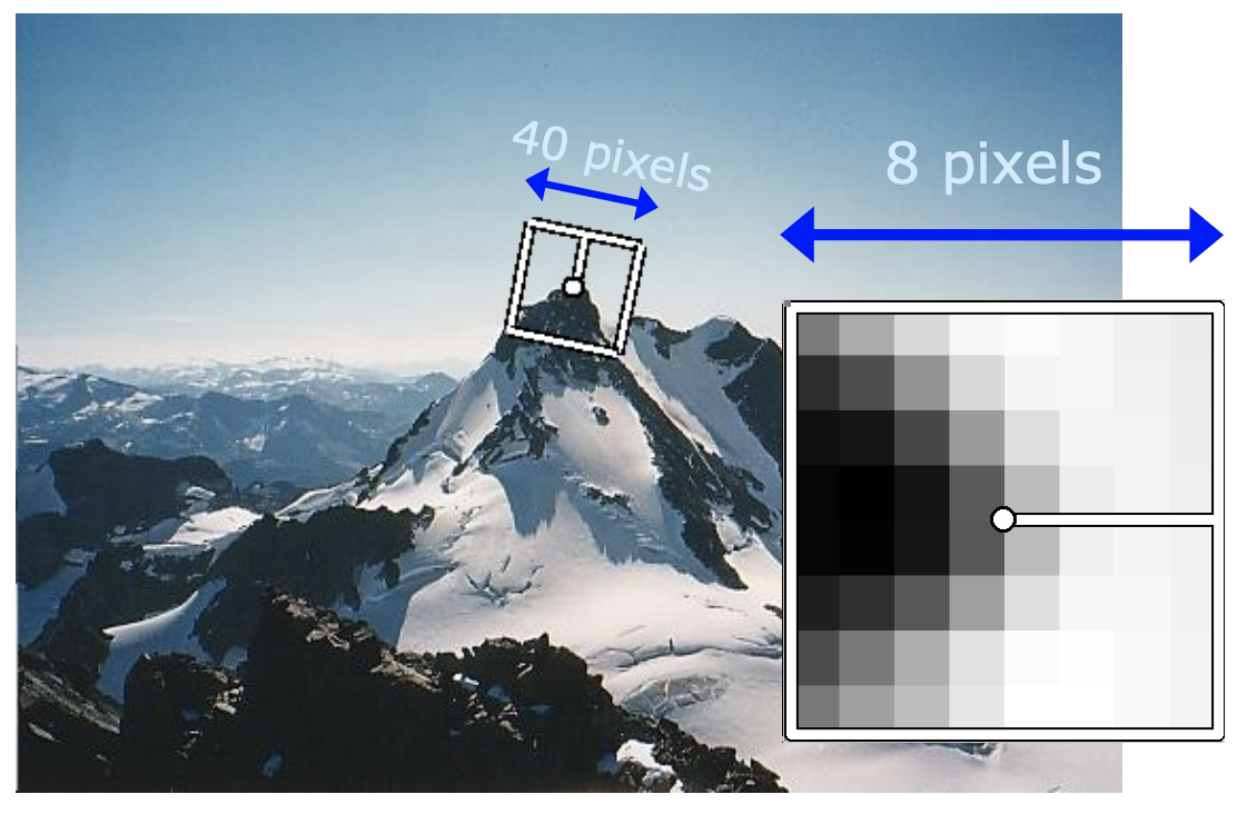Feature descriptor extraction example

Matching Feature Descriptors

Now that we have extracted the feature descriptors, we can approximate the point matches between the left and right images using a very simple algorithm. For every feature descriptor on the left image, we compute the squared Euclidean (L2) distance between it and every feature descriptor on the right image. These distances represent how similar two descriptors are. Once we have computed all the L2 distances from the current left descriptor to all right descriptors, we need to figure out a metric to determine the best match. Intuitively, we could have deduced than the best match is the descriptor with the shortest distance, but it turns out this is not the case. According to the research paper Multi-Image Matching using Multi-Scale Oriented Patches by Matthew Brown et al. (available here) from which this part of the project is mostly based, suggests that the ratio between the first and the second nearest descriptors provides a better metric than choosing the closest match. Therefore, it is suggested a pre-defined threshold value less than 0.6. For this project we set out threshold between 0.3 and 0.4. The figure below shows the distributions of matching error for correct and incorrect matches.

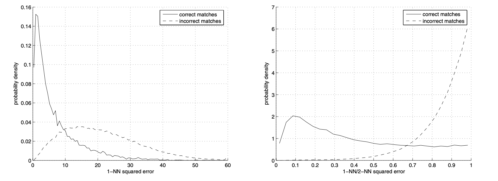Note that the distance of the closest match (the 1-NN) is a poor metric for distinguishing whether a match is correct or not (figure a), but the ratio of the closest to the second closest (1-NN/2-NN) is a good metric (figure b). (Matthew Brown et al.)

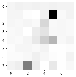
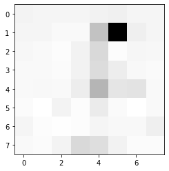
Some matching feature descriptors are shown below. As we can see they are remarkably similar. For this project, we do not apply rotation invariance to the descriptors as we assume both images to be stitched to be oriented in the same way.

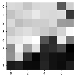Feature Descriptor example.		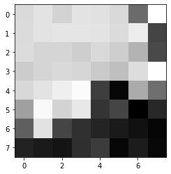Feature Descriptor example.		Feature Descriptor example.		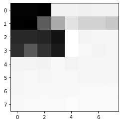Feature Descriptor example.
Feature Descriptor example.		Feature Descriptor example.		Feature Descriptor example.		Feature Descriptor example.

The resulting pre-matched Harris points for our test images are the following:

Matched Feature descriptors.

Matched Feature descriptors.

PART B4: Random Sample Consensus (RANSAC)

Although we have a decent set of pre-matched points, we one problem: the number of matched points is not guaranteed to coincide as shown in the previous part. In addition, we may face the scenario that multiple feature descriptors’ points can match even though they may not even be the ground truth correspondence points! This is solved by another simple but clever algorithm known as Random Sample Consensus (RANSAC). The basic idea is to randomly sample 4 feature point pairs from our pre-matched feature descriptors, compute a homography transformation between them, compute the number of transformed left points that best approximate the right points while falling below a predefine threshold (setting 1-3 pixels threshold produce good results). We repeat this process a certain number of times (500 times, for example) and finally we choose the largest set of satisfied points (known as inliers). This resulting point set consist of the matched points between the two images as shown below.

Correspondence points.

Correspondence points.

Autostitching

PART B5: Autostiching for mosaicing

Finally, we use our final matching points to compute the homography transformation which is then used by our stitching algorithm. The results are pretty satisfying! We show some examples below.

Manual Stitching

Automatic stitching

Manual Stitching

Automatic stitching

Manual Stitching

Automatic stitching

Manual Stitching

Automatic stitching

Final Thoughts

Part A

As the culmination project of CS192-26, we used much of what we learned in projects 2 and 3 for the implementation of this project, plus ingenious mathematical machinery that allowed us to warp and blend two images into a nice mosaic. Image transformations are without doubt an extremely important workhorse in the image processing field. Their possibilities are boundless!

Part B

For the contemporary computer scientist, finding ways to solve image recognition problems usually involves some sort of machine learning artillery. However, in this project we have demonstrated that not every problem should be solved with heavy-duty AI approaches like we did in project 4 for facial landmark detection. Finding correspondence points is a quite easy task for humans to do, but for computers is not that obvious. They need a bit more insight about the problem. In this project, we delved on the mathematics behind image warping, rectification, blending and mosaicing for part A. However, to solve the problem of point matching in part B required us to resort to some clever algorithms based mostly on pure linear algebra and with a hint of calculus: Harris Corner Detector, Adaptive Non-Maximal Suppression (ANMS), a simplified version of Multi-Scale Oriented Patches (MOPS), and Random Sample Consensus (RANSAC), which produced outstanding results. This project provided us with a significant amount of both coding and mathematical experience, and it has sparked our interest and appreciation on the image processing field even more! Let’s see what the future of image processing and computer vision brings to the world!