
Overview
Continuing our image manipulation journey, we now explore the fascinating world of image morphing, which refers to the process of distorting one image into another. In this project we present a technique to morph faces through a seamless animated transition using Delaunay tessellation, B-spline/bilinear interpolation/rounding, linear mapping (exclusively affine transformations), and alpha crossfading (aka. weighted averaging). In addition, we analyze sets of faces to extracts the mean facial shape to produce interesting results that challenge our perception of the real world.
The idea behind morphing images
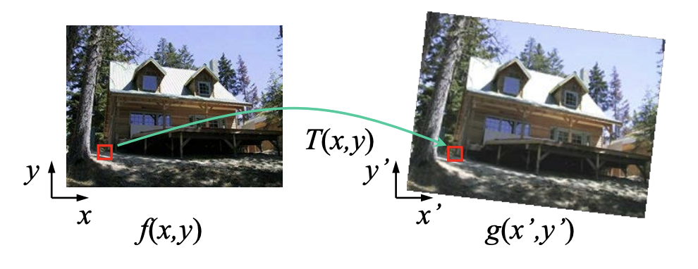
The basic idea behind warping and morphing can be easily explained geometrically. Imagine we have two 2D triangles: Triangle A with vertices (a, b, c) and Triangle B with vertices (a’, b’, c’). Each triangle defines a basis for the plane spanned by their vertices. Now suppose we have a point P inside triangle A with coordinates (x, y) in basis A, and we are interested in knowing the relative position of point P inside the triangle B. We call this point P’ with coordinates (x’, y’) in basis B. To achieve this, we want to compute a transformation T to map points from one basis into the other se we can transform (warp) our point P in basis A into point P’ in basis B. This process is represented in the following diagram.
|
We are interested in finding the transformation T. |
In order to compute this transformation matrix T, we use the vertices from both triangles (the basis vectors of the spaces they span) to construct two matrices, which then will be used to compute the transformation T by applying one inverse operation in A and one dot product operation as shown in the equation below.
|
The resulting matrix T is known as an affine transformation matrix. |
The resulting matrix T is known as an affine transformation matrix, which can translate, scale, rotate, and shear shapes while preserving lines and parallelism but not necessarily distances and angles. We can get point P’ = (x’, y’) inside Triangle B from point P = (x, y) inside triangle A by simply applying the transformation T as P’ = T ⋅ P
|
P(x', y') = T ⋅ P(x, y) |
How will this schema help us to go create a hybrid (morphed) image between two images? Well, we already know how to map points from one triangle into another, and this will become really handy in the following example. Suppose that our triangles A and B are triangular sections of two images and each coordinate inside these triangles have an RGB color value assigned to it. To generate a hybrid image, we want to compute an averaged RGB color value for every corresponding coordinate in tringle A and triangle B and save in triangle C. This intermediate triangle C is constructed by averaging the vertices of triangles A and B. To compute the values for C, we need to figure out the corresponding coordinates between A and C and between B and C. For this, we compute two transformations: T1 which transforms points from A to C, and T2 which transforms points from B to C. Ideally, we could just transform coordinates from A to C and B to C and set averaged RGB color values from A and B values into C. This is known as “forward warping.”
 Mapping from source images to target image might leave "empty" spots. |
However, when we map corresponding coordinates from A and B into C there is a high chance that not all coordinates in C will be touched. Fortunately, we can work around this problem by “inverse warping” (i.e. transforming) the coordinates from C into both A and B. In this way, we guarantee that every coordinate in triangle C will have access to RGB values from both triangles A and B to compute their average.
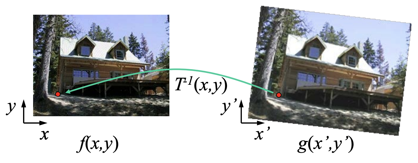 Mapping from target image to source images guarantess no "empty" spots. |
This almost solve our mapping problem, but since pixel coordinates inside each triangle are discrete, we need to find a way to get RGB values for any transformed, non-discrete coordinate from C. We can use B-spline, bilinear interpolation, or rounding to approximate the best value for that transformed coordinate.
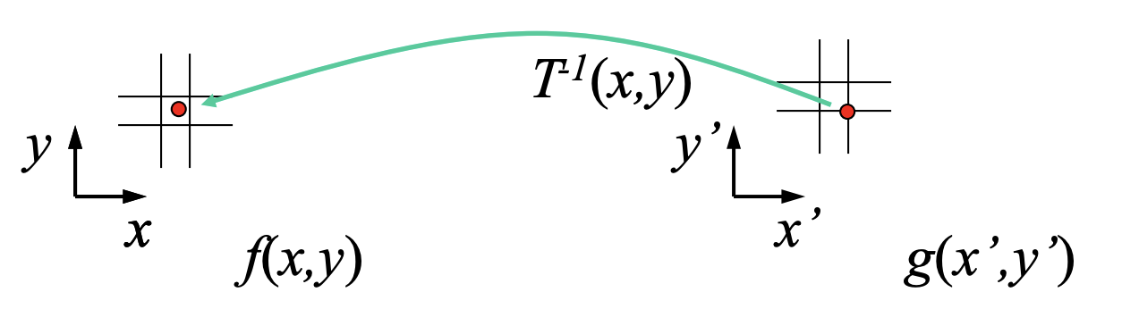 We need to approximate the pixel value using B-spline, bilinear interpolation, or rounding to nearest pixel. |
We decided to round coordinates to the nearest pixel since this produces fairly good, fast, and easy to compute results! Now we are able to combine (morph) two triangular sections of our images. We can repeat the process for their remaining area of the two images to get the full morphed hybrid! Next, we explain a bit more on how this is done.
PART 1: Computing the "Mid-way Face"
Part 1.1: Defining Correspondences
We already know how to morph triangles, so we just need to dive up our source images into triangles and voila! we can now morph all triangle segments individually to get our morphed image! Our problem is now reduced in finding the best way to segment our images. We can use a triangle mesh to dive our image into triangular segments. In order to define a good triangle mesh, we need to make sure all the important features are enclosed by many small triangles. Since we will work on faces, we need a dense mesh of triangles around eyes, mount, nose, and eyebrows as these features define the appearance of a person. We could, in principle, manually define a mesh over the faces to be morphed, making sure that each triangle in one image has a corresponding triangle in the other one. However, while this approach is valid it is very cumbersome. Fortunately, there is an easier way to generate triangle meshes using Delaunay tessellation (triangulation). Given an array of 2D points, a Delaunay triangulation will return a set of vertex indices (for the given arrays) defining triangles, while ensuring the circumcircle associated with each triangle contains no other point in its interior. Examples of good and bad Delaunay triangulations are shown below.
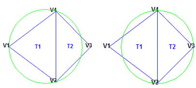 No point (vertex) is inside the circumcircle associated with each triangle. |
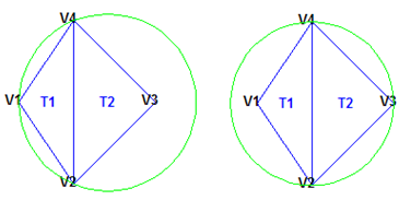 There are points (vertex) inside the circumcircle associated with each triangle. |
Delaunay triangulation maximizes smallest angles so that we avoid really thin triangle that would otherwise result into weirdly morphed results. To apply this algorithm in our images we first need to define a set of correspondence points between the two images. We decided that 58 points generate excellent results). Each point in image 1 will have a “twin” point in image 2. For this project, all correspondence pairs are defined manually using a custom-made utility. These points are stored into an array and saved into a file. Then we use points from the two images to compute an averaged point set (the midway shape) which will be the input for the Delaunay tessellation algorithm. Using the resulting triangle indices, we can obtain a neat triangle mesh for each image that will be used for our morphing algorithm defined above. We use will use Scikit-image draw.polygon to get a numeric Boolean mask of the same size as the source image. It takes the vertex coordinates of a triangle and returns a matrix where every value is zero except all pixels that lie inside of the given triangle. This will be useful to define the target RGB color value position in our final morphed image. Some examples of correspondence points and their associated triangle mesh are shown below.
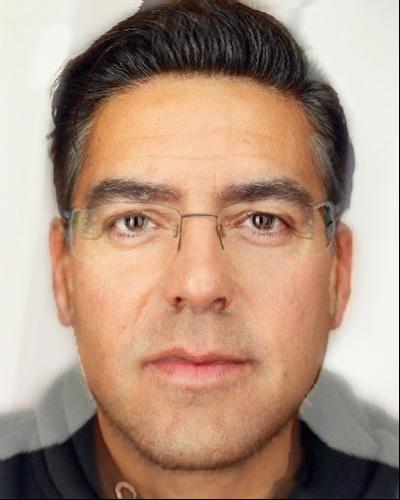
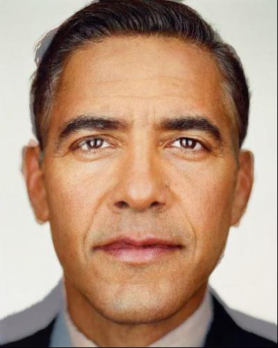
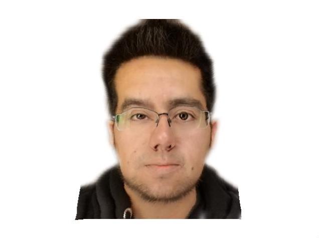
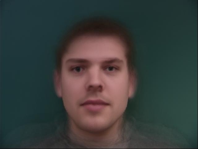
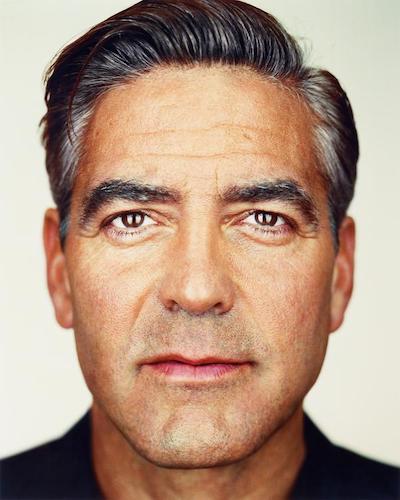 Original image. |
 Original image. |
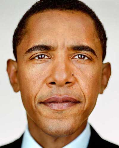
 Original image. |
||
 Each individual point was set manually. |
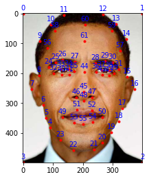 Each individual point was set manually. |
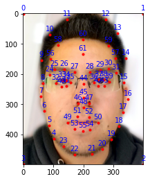 Each individual point was set manually. |
||
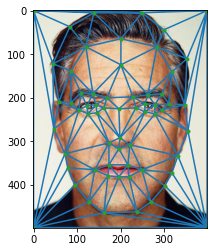 This triangle mesh was computed using the point mean between the two source images to be morphed as input for the Delaunay triangulation |
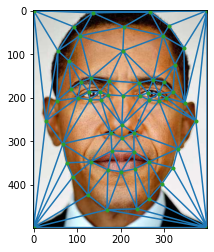 This triangle mesh was computed using the point mean between the two source images to be morphed as input for the Delaunay triangulation |
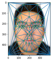 This triangle mesh was computed using the point mean between the two source images to be morphed as input for the Delaunay triangulation |
Note: The triangle mesh for the previous images was computed using the point correspondence average from the two source images to be morphed as the input for the Delaunay triangulation. In this example, the pairs to be morphed are George-Author (me), George-Obama, and Obama-Author (me). Note that each face mesh has exactly the same number of triangles and that the relative position of each one is consistent among the three images.
Part 1.2: The "Mid-way Face"
Now we apply our complete morphing algorithm on each face pair (and their respective meshes) to get the following mid-way morphed faces.
 Morphed (hybrid) result at 50% (midway). |
 Morphed (hybrid) result at 50% (midway). |
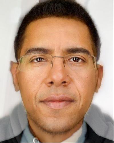 Morphed (hybrid) result at 50% (midway). |
PART 2: The Morph Sequence
Our next goal will be generating a sequence of morphed faces such that we start with one of the original faces, then we go through a series of morphed phases to arrive to the mid-way face, and the we continue morphing until we reach the second original face. In the previous example, we warped each mesh triangle into the mean shape of the two source faces, where they contributed exactly 50% of their shape (point coordinates) and appearance (RGB color). Now we are interested in generating a sequence of frames where we start with one face contributing 100% in both aspects (shape and appearance) and the second one with 0% contribution, then reaching 50%/50% contribution (the mid-way face), and finally reaching the end of the sequence with the first image contributing 0% and the second image with 100% in both aspects. In other words, we need to use weighted averaging with parameter t ∈ [0, 1] to indicate the level of contribution from each image, the following equation defines the level of contribution for every aspect. For the appearance aspect this is call alpha-crossfading (cross-dissolve) where α = t.
 This is used to define the warp and cross-dissolve contributions from each image. |
The morphing algorithm can be summarized in the following steps:
- Define the correspondence points on each image making sure they are defined in the same order.
- Compute the mean shape from the correspondence points.
- Use the mean to compute the Delaunay triangulation that will be used in both images.
- For every t ∈ [0, 1]:
- Compute the average shape at t (weighted average of triangle vertices).
- For each triangle in mesh:
- Get the affine projection to the corresponding triangles in each image.
- For each pixel in the target triangle, find the corresponding points in each image and set value to weighted average (crossdissolve RGB pixels values).
- Save morphed image (frame).
We generate a sequence of 50 frames from face to face and then we combine the results into the animation shown below.
 Morphing animation. 50 frames (25 frames per second) |
 Morphing animation. 50 frames (25 frames per second) |
 Morphing animation. 50 frames (25 frames per second) |
PART 3: The "Mean face" of a population
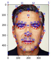
One interesting application of our morphing algorithm is to find the mean face of a face dataset. We use the Danes face dataset provided here. We will use 40 pictures of frontal, neutral faces for our analysis. This sample population includes 33 male pictures and 7 female pictures. The dataset is already annotated so we imported the datapoints provided to set up correspondences and Delaunay triangulations. We have created a little function that removes unwanted pictures, parse the datapoints files, and shows the order in which points were defined. This information becomes handy when manually selecting points for additional non-annotated images. The order or points is shown below. Note: the first 4 points corresponds to the four corners (not shown).
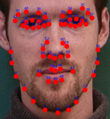 Numbering on the points was not provided but automatically computed instead. |
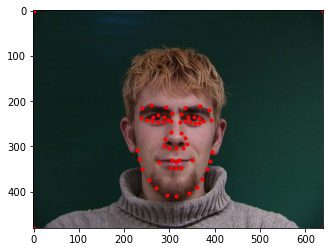
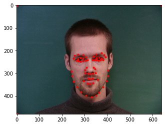
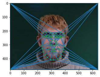
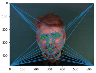
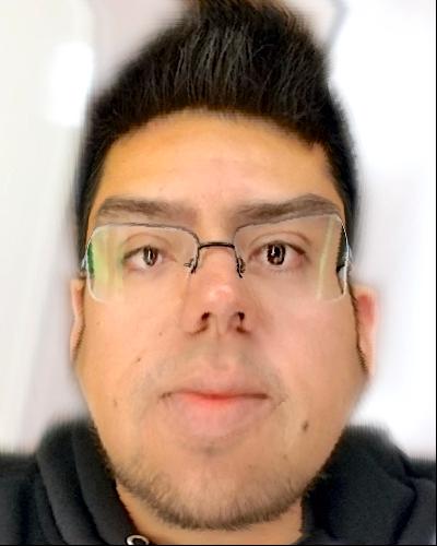
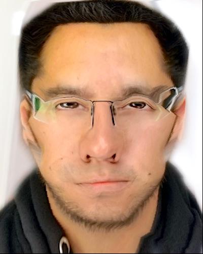
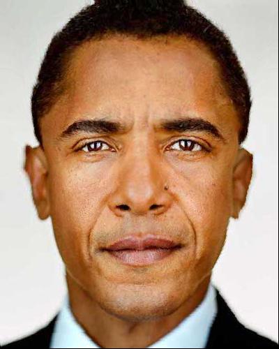
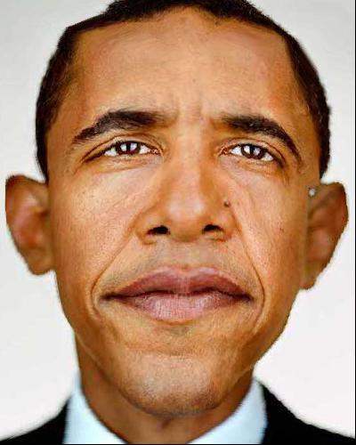
Here are some examples from the dataset plus a picture of the author (me), their correspondence points, and Delaunay triangulations.
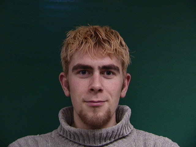 Face from Danish dataset. |
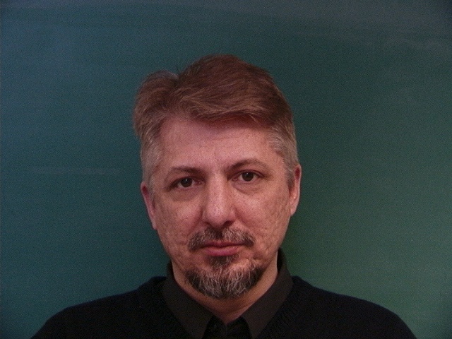 Face from Danish dataset. |
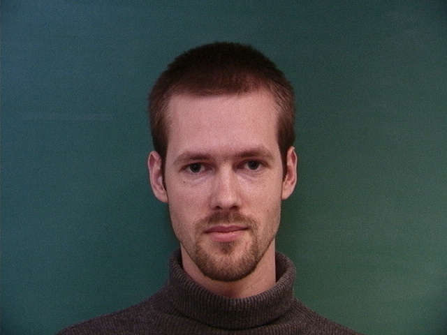 Face from Danish dataset. |
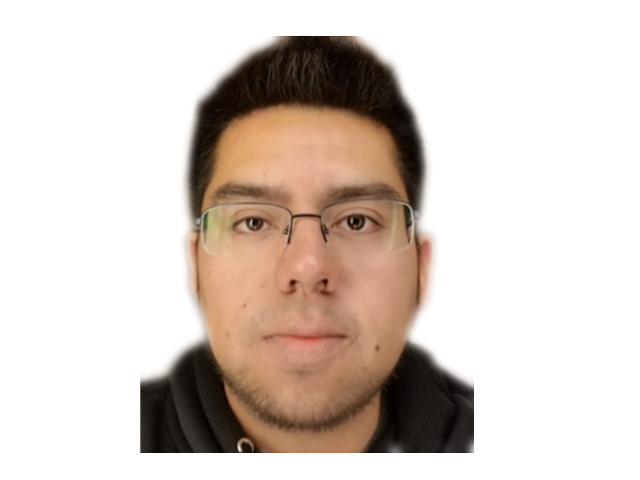 Author's face. |
|||
 Face from Danish dataset. |
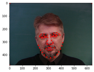 Face from Danish dataset. |
 Face from Danish dataset. |
 Author's face. |
|||
 Face from Danish dataset. |
 Face from Danish dataset. |
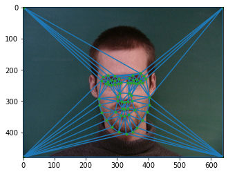 Face from Danish dataset. |
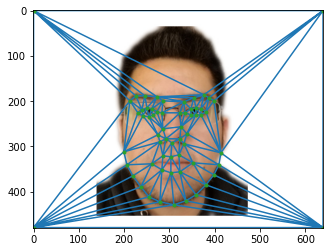 Author's face. |
To compute the mean face, we compute the mean shape by averaging the datapoints of all 40 faces. The process is similar to the one used in part 1 of this project. Once we have computed the mean shape, we morph every face into it while taking only 1/40 of the their RGB color values (1/40 cross-dissolve factor). The resulting face is the representation of all faces warped and cross-dissolved to the mean shape.
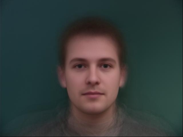 Result of morphing all images together at the midways shape. |
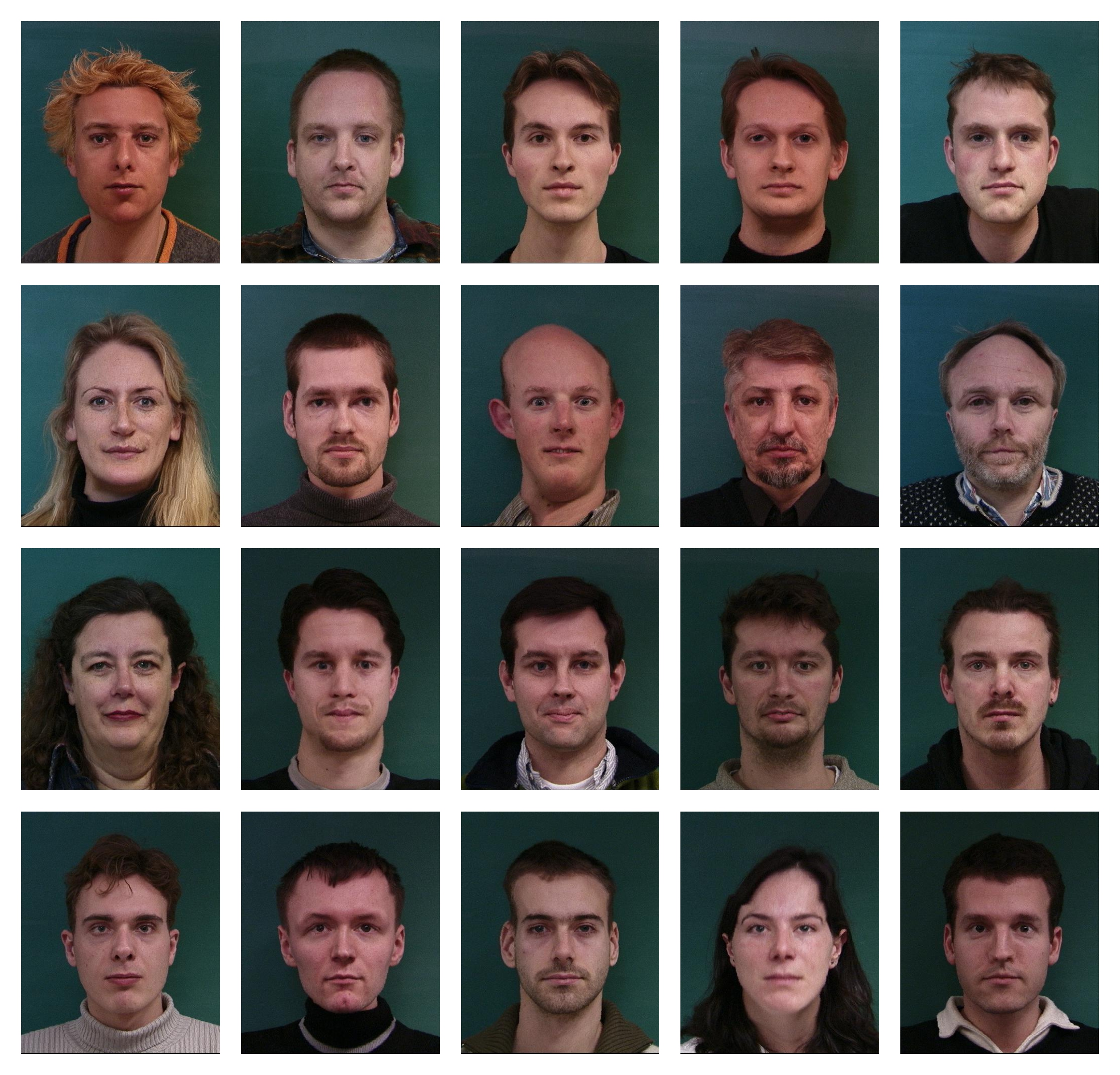
Now we can play around by morphing each face into this mean face. We present some examples down below. Note that some not all faces morph pleasantly into the mean. This is expected since there are people with unique facial characteristics and facial shapes. First we show the original faces.
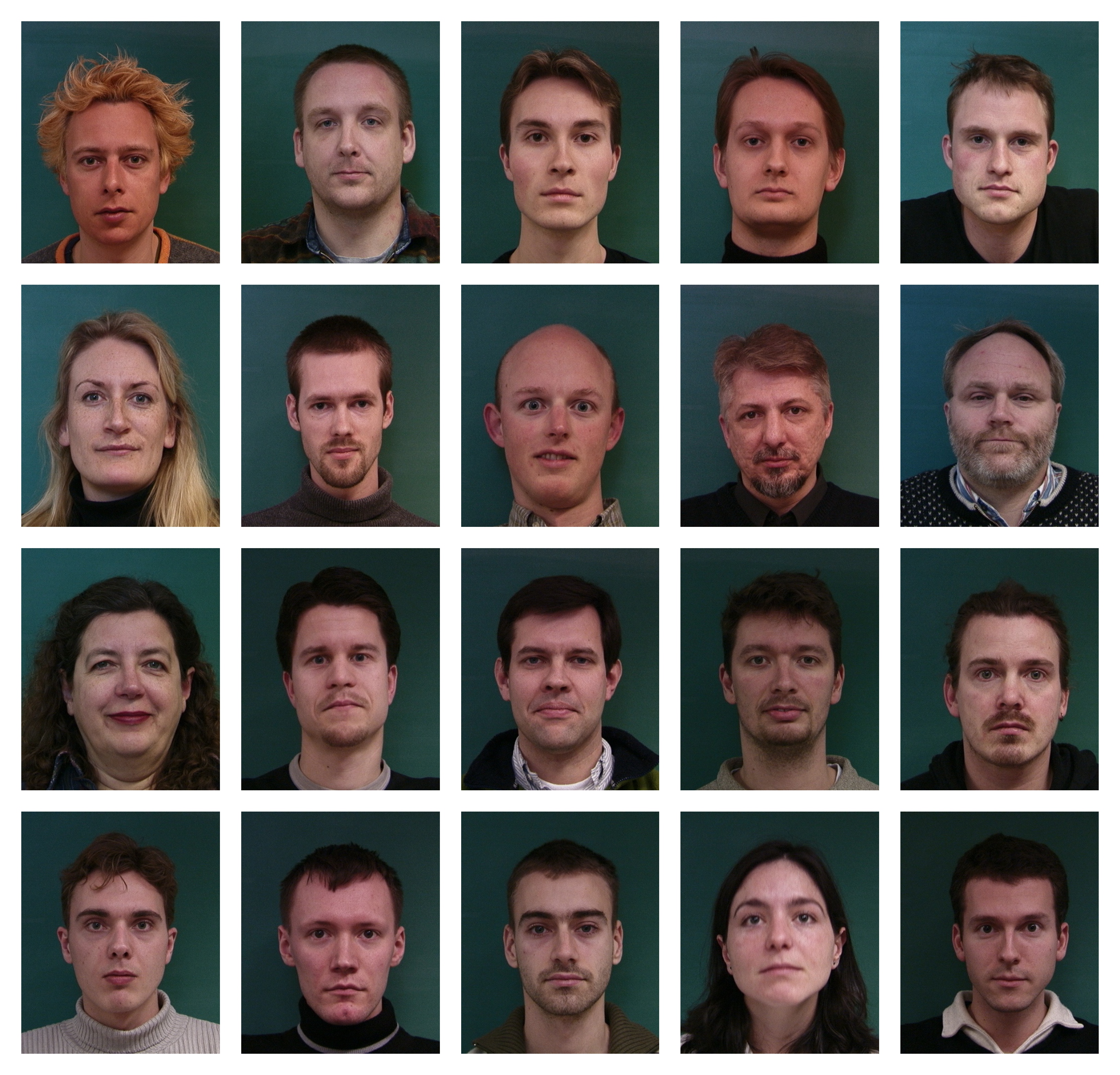 Original faces. |
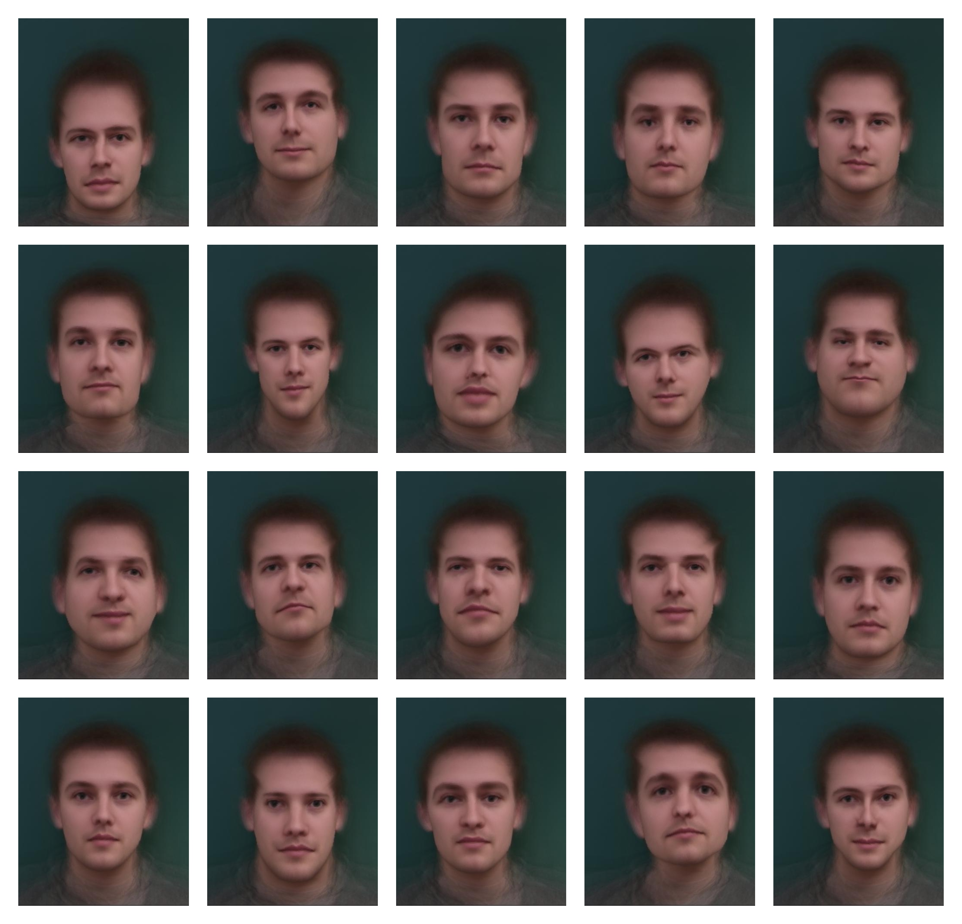
Here are the same faces morphed into the mean shape.
 Every face now share similar geometry. |
We can do the opposite by morphing the resulting mean face into each face shape. This usually generates more pleasant results as shown below.
 The mean face morphed into every geometrical face shape. |
We finally present the results of my face under the same experiments from above. It seems the author's face does not match really well with Danish appearance!
|
Original face. |
 Face to mean. |
 Mean to face. |
Creating a custom-made face dataset
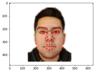
In addition to this provided dataset, we present an entirely custom-made “Celebrities” face dataset featuring photos from Martin Schoeller, a New York-based photographer whose style of "hyper-detailed close ups" is distinguished by similar treatment of all subjects whether they are celebrities or unknown (Wikipedia), and other pictures with similar style. Each image was manually aligned and annotated to produce a dataset which could be bulk processed just like the Danish dataset. This dataset used 58 points per image, some annotated examples are shown below.
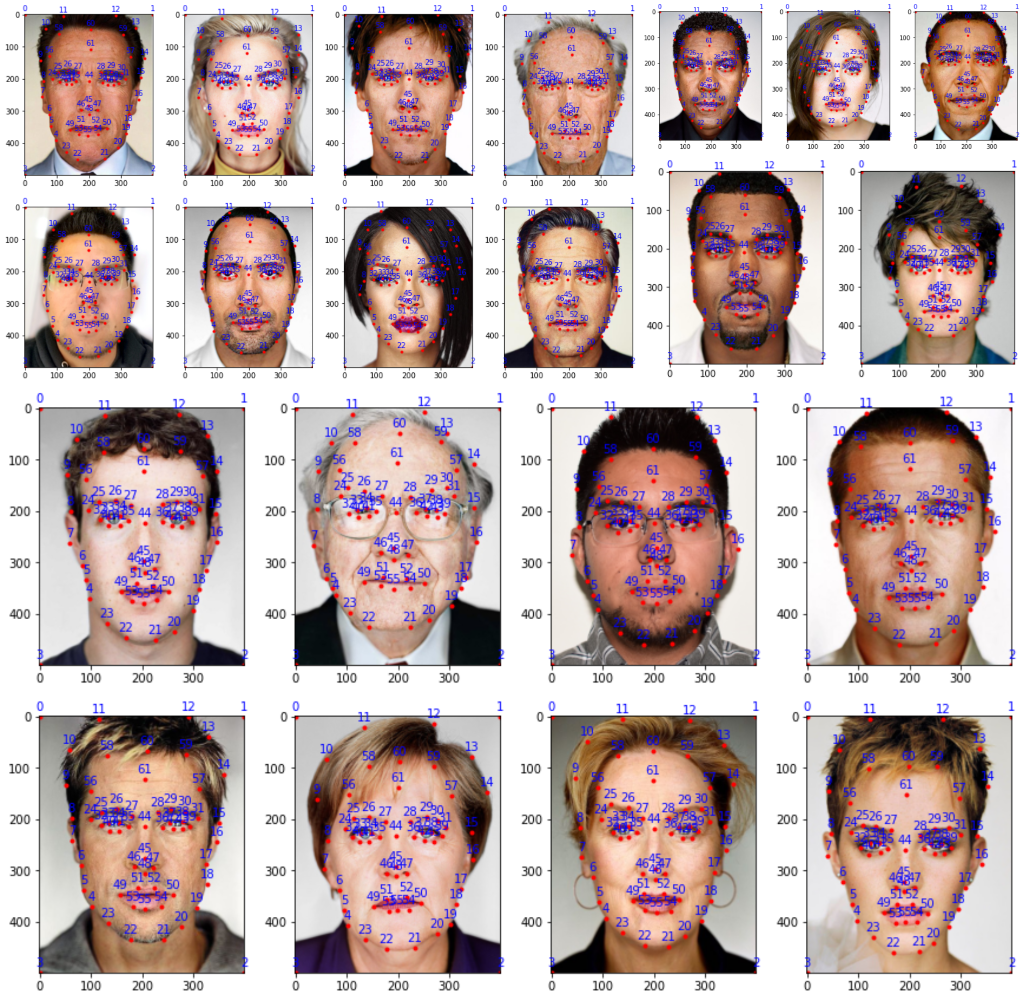 Every face was manually annotated. |
The mean face from this dataset features light skin color and very symmetrical semblance.
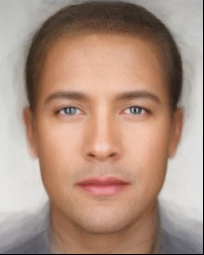 The mean face features blue-ish eyes, rounded mouth, and symmetrical appearance. |
In a similar way as with the Danes dataset, we show the original images, followed by results from morphing each Face into the mean, and the mean into each face. First, we show the original pictures.
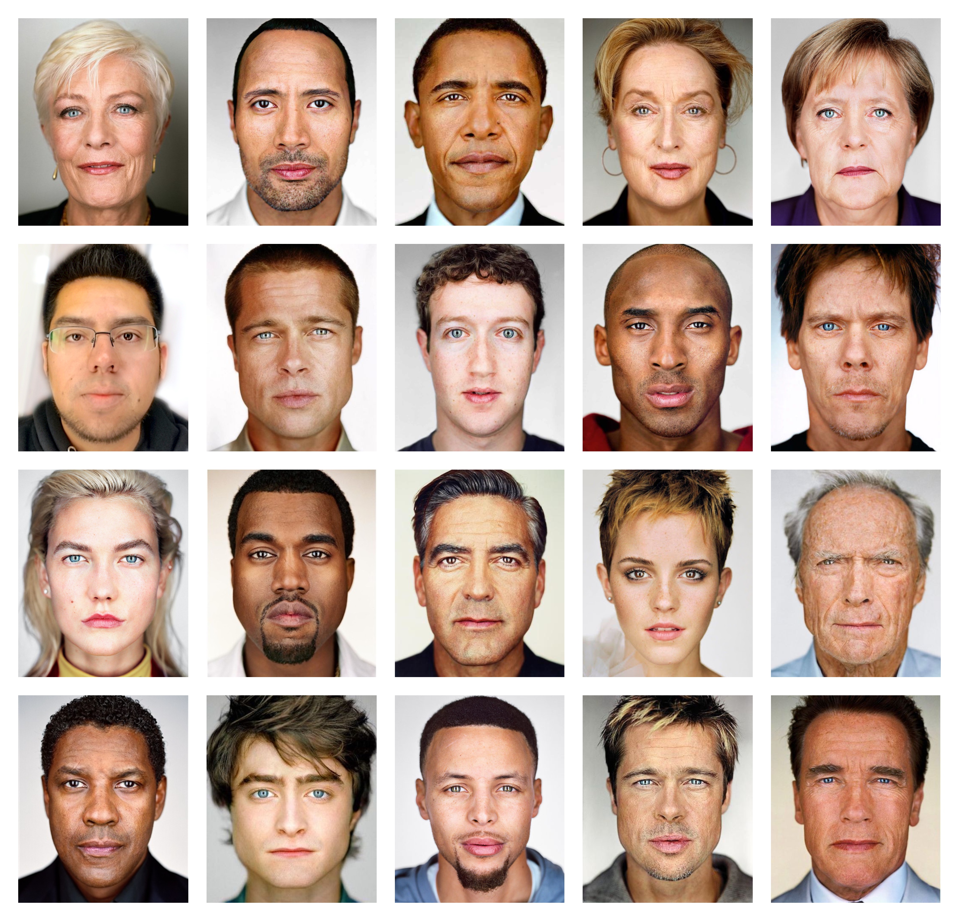 Original faces. |
Here we show the results of morphing each face into the Celebrity mean face.
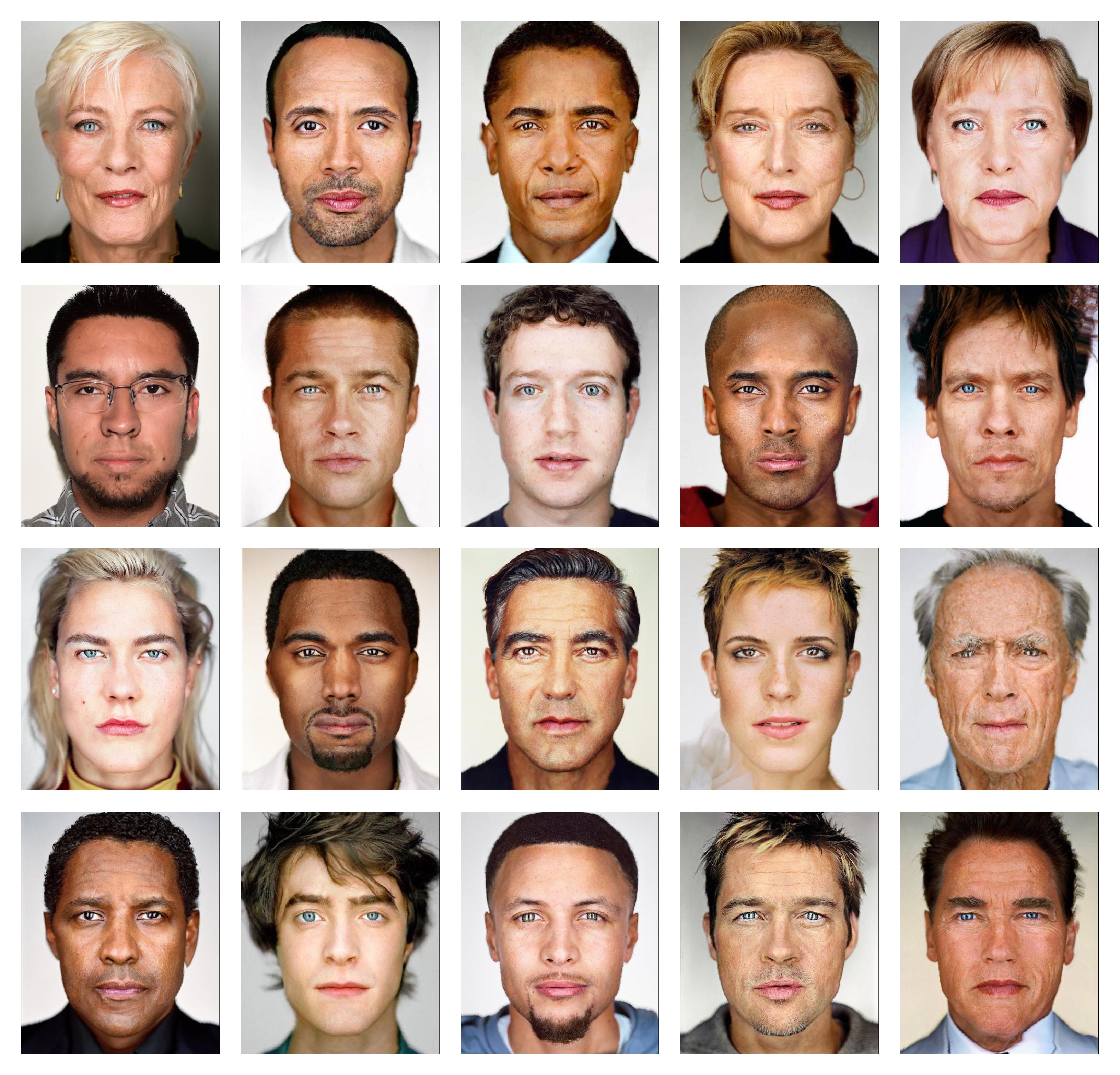 Every face now share similar geometry. |
Finally, we do the opposite by morphing the resulting mean face into each Celebrity face shape.
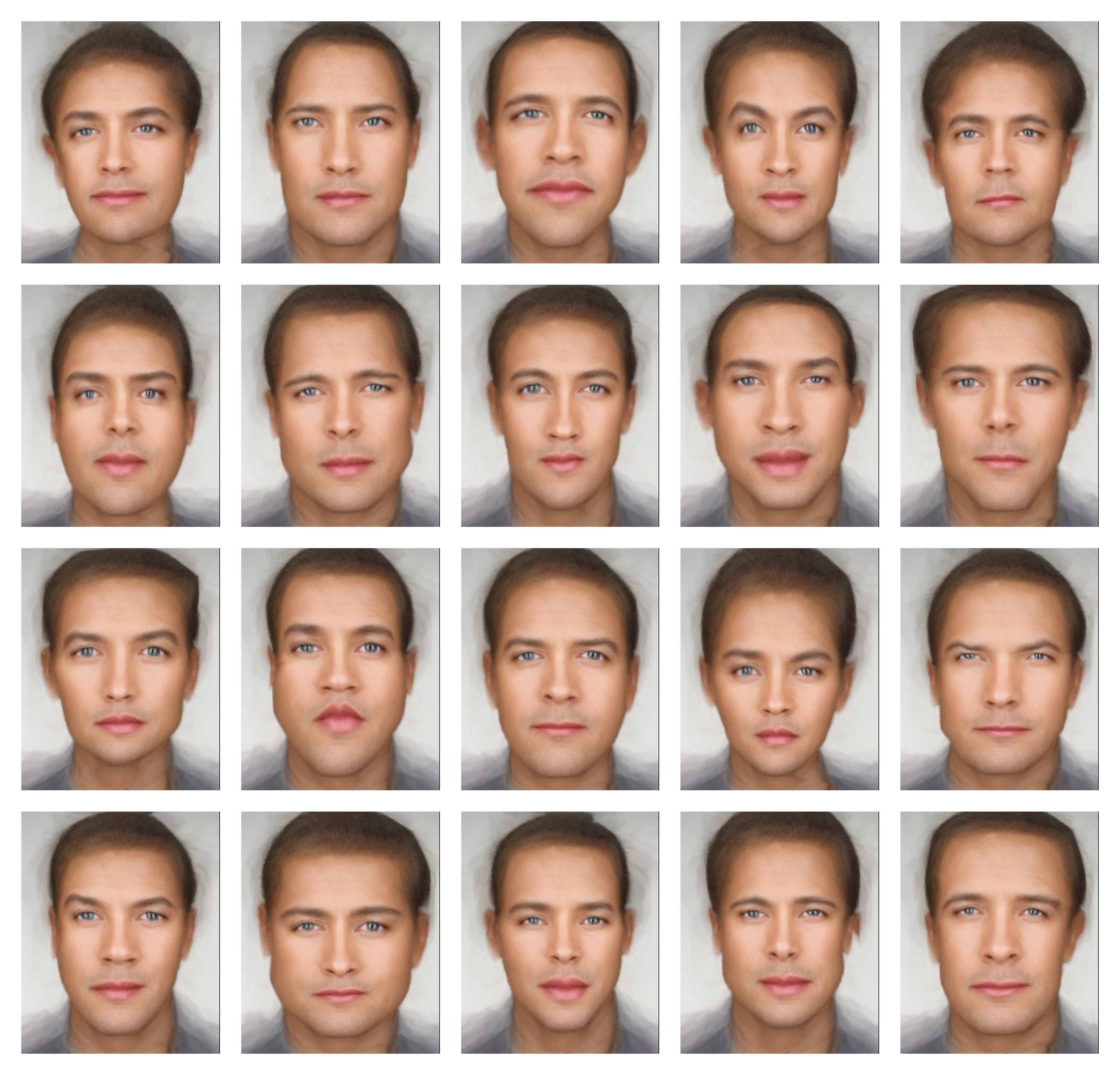 The mean face morphed into every geometrical face shape. |
PART 4: Caricatures: Extrapolating from the mean
To create caricatures, we extrapolate from the mean shape as follow: take the difference between the source face and target mean, then add back to the mean the computed difference multiplied by a factor α (alpha). Some examples are shown below.
 A fun caricature! |
 A fun caricature! |
 A fun caricature! |
 A fun caricature! |
Bells and Whistles
Ethnicity swap
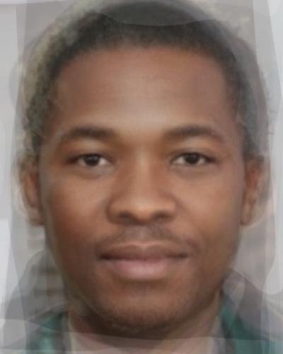
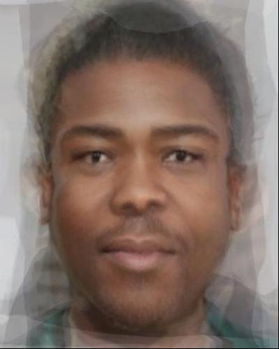
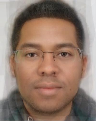
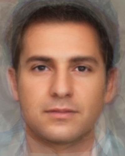
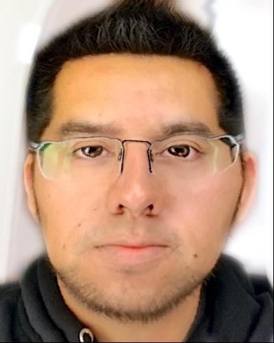
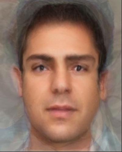
Yet another application of morphing and face averaging is to generate "ethnicity swaps.” We can approximate what a face would look like using the mean face of a given ethnic or racial group. In this example we will be swapping the author’s face, a Mexican-born male, into the mean Taiwanese male, mean South African male, and mean Italian male. The results are displayed below.
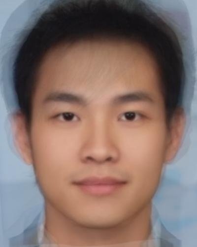 Mean face |
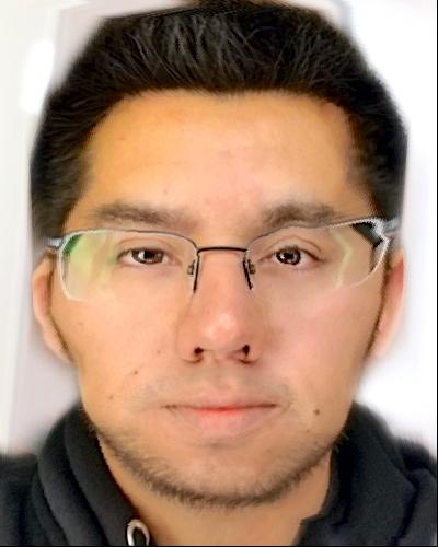 My face morphed to mean shape. |
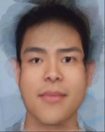 Mean face morphed into my face shape. |
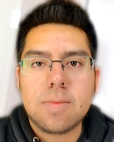 Original face |
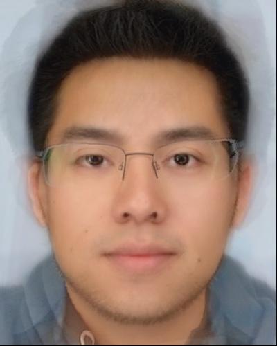 Ethnicity swap |
||||
 Mean face |
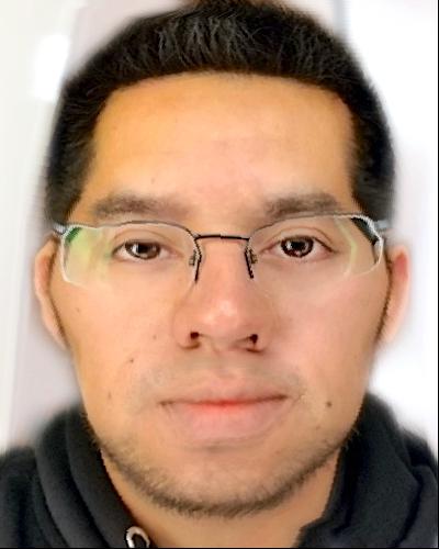 My face morphed to mean shape. |
 Mean face morphed into my face shape. |
Original face |
 Ethnicity swap |
||||
 Mean face |
 My face morphed to mean shape. |
 Mean face morphed into my face shape. |
Original face |
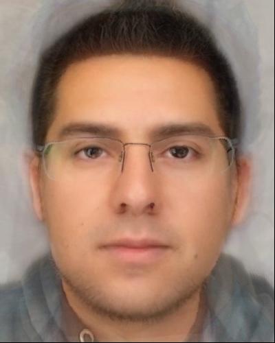 Ethnicity swap |
Musical morphing sequence
Finally, we use the custom-made dataset to create a dramatic morphing sequence! And with this video we conclude another interesting and fun adventure into the thrilling world of image processing!
Final thoughts
In this project we explored how 2D transformations can produce some interesting effects on images and we surveyed some practical applications. This project was very entertaining and challenging at the same time. Let’s see what other CS194-26 adventures are waiting for us!